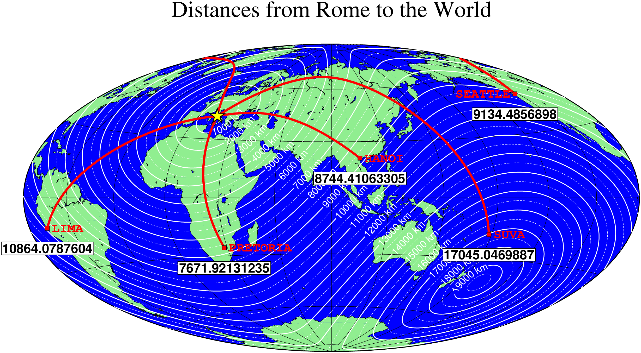
(23) All great-circle paths lead to Rome
While motorists recently have started to question the old saying “all roads lead to Rome”, aircraft pilots have known from the start that only one great-circle path connects the points of departure and arrival 1. This provides the inspiration for our next example which uses grdmath to calculate distances from Rome to anywhere on Earth and grdcontour to contour these distances. We pick five cities that we connect to Rome with great circle arcs, and label these cities with their names and distances (in km) from Rome, all laid down on top of a beautiful world map. Note that we specify that contour labels only be placed along the straight map-line connecting Rome to its antipode, and request curved labels that follows the shape of the contours.
The script produces the plot in Figure; note how interesting the path to Seattle appears in this particular projection (Hammer). We also note that Rome’s antipode lies somewhere near the Chatham plateau (antipodes will be revisited in Example (25) Global distribution of antipodes).
using GMT

lon  = 12.50
lat  = 41.99
Gdist = gmt("grdmath -Rg -I1 12.5 41.99 SDIST")

coast(region=:global, land=:lightgreen, ocean=:blue, shore=:thinnest, area=1000,
      frame=(grid=30, title="Distances from Rome to the World"),
      proj=(name=:Hammer, center=90), figsize=20, portrait=false)
grdcontour!(Gdist, annot=(int=1000, labels=(curved=true, unit="\" km\"", font="white")),
            labels=(line="Z-/Z+",), smooth=8, cont=500,
            pen=((contour=true,pen="thinnest,white,-"), (annot=true, pen="thin,white")) )

# Location info for 5 other cities + label justification
cities = [105.87 21.02; 282.95  -12.1; 178.42 -18.13; 237.67 47.58; 28.20 -25.75];
just_names = ["LM HANOI", "LM LIMA", "LM SUVA", "RM SEATTLE", "LM PRETORIA"];
D = mat2ds(cities, just_names)

# For each of the cities, plot great circle arc to Rome with gmt psxy
plot!([lon lat; 105.87 21.02], lw=:thickest, lc=:red)
plot!([lon lat; 282.95 -12.1], lw=:thickest, lc=:red)
plot!([lon lat; 178.42 -18.13],lw=:thickest, lc=:red)
plot!([lon lat; 237.67 47.58], lw=:thickest, lc=:red)
plot!([lon lat; 28.20 -25.75], lw=:thickest, lc=:red)

# Plot red squares at cities and plot names:
plot!(cities, marker=:square, ms=0.2, fill=:red, markerline=:thinnest)
text!(D, offset=(away=true, shift=(0.15,0)), font=(12,"Courier-Bold",:red),
      justify=true, no_clip=true)

# Place a yellow star at Rome
plot!([12.5 41.99], marker=:star, ms=0.5, fill=:yellow, ml=:thin)

# Sample the distance grid at the cities and use the distance in km for labels
dist = grdtrack(Gdist, D);
text!(dist, offset=(0, -0.5), noclip=true, fill=:white, pen=true, clearance=0.05,
      font=(12,"Helvetica-Bold"), justify=:CT, zvalues="%.0f", show=true)
These docs were autogenerated using GMT: v1.33.1