using GMT
resetGMT() # hide
# Data obtained via website and converted to netCDF thus:
# curl http://www.antarctica.ac.uk//bas_research/data/access/bedmap/download/bedelev.asc.gz
# gunzip bedelev.asc.gz
# grdreformat bedelev.asc BEDMAP_elevation.nc=ns -V
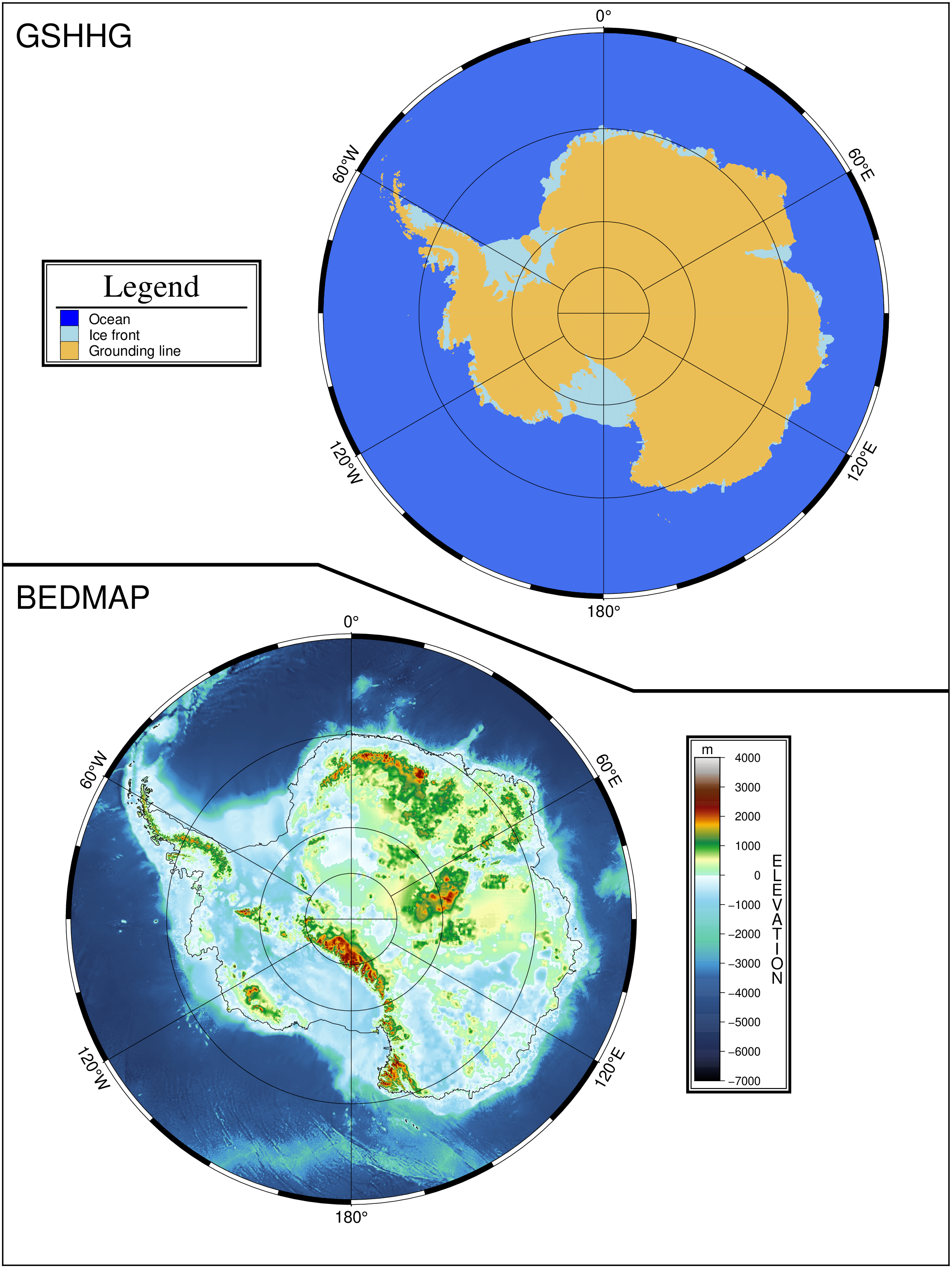
makecpt(cmap=:earth, range=(-7000,4000))
grdimage("@BEDMAP_elevation.nc", frame=:none, proj=:linear, figscale="1:60000000", nan_alpha=true)
coast!(region=(-180,180,-90,-60), frame="afg", proj=(name=:stere, center=(0,-90), parallel=-71),
figscale="1:60000000", shore=0.25)
colorbar!(pos=(inside=true, anchor=:RM, length=(6.4,0.5), offset=(1.25,0), justify=:LM, neon=true),
box=(pen=true, inner=true), xaxis=(annot=1000, label=:ELEVATION), ylabel=:m)
# GSHHG
coast!(land=:lightblue, water=:royalblue2, frame="none", xshift=5, yshift=12)
coast!(land=:lightbrown, frame="afg", area="+ag")
legend!(region=(-180,180,-90,-60), box=(pen=true, inner=true),
pos=(inside=true, anchor=:LM, width=4.3, justify=:RM, offset=(1.25,0)),
mat2ds(["H 18p,Times-Roman Legend"
"D 0.1i 1p"
"S 0.15i s 0.2i blue 0.25p 0.3i Ocean"
"S 0.15i s 0.2i lightblue 0.25p 0.3i Ice front"
"S 0.15i s 0.2i lightbrown 0.25p 0.3i Grounding line"])
)
# Fancy line
plot!(region=(0,7.5,0,10), proj=:linear, figscale=2.5, frame=:bare, lw=2,
xshift=-6.35, yshift=-13.3,
[0 5.55
2.5 5.55
5.0 4.55
7.5 4.55])
text!(text_record([0 5.2; 0 9.65], ["BEDMAP", "GSHHG"]), font=18, justify=:BL,
offset=(away=true, shift=(0.25,0)), show=true)