using GMT
GMT.resetGMT() # hide
G = earthtide(T="2022-07-07T12:00:00");
imshow(G, coast=true, colorbar=true, title="Earth tide at noon 7-July-2022")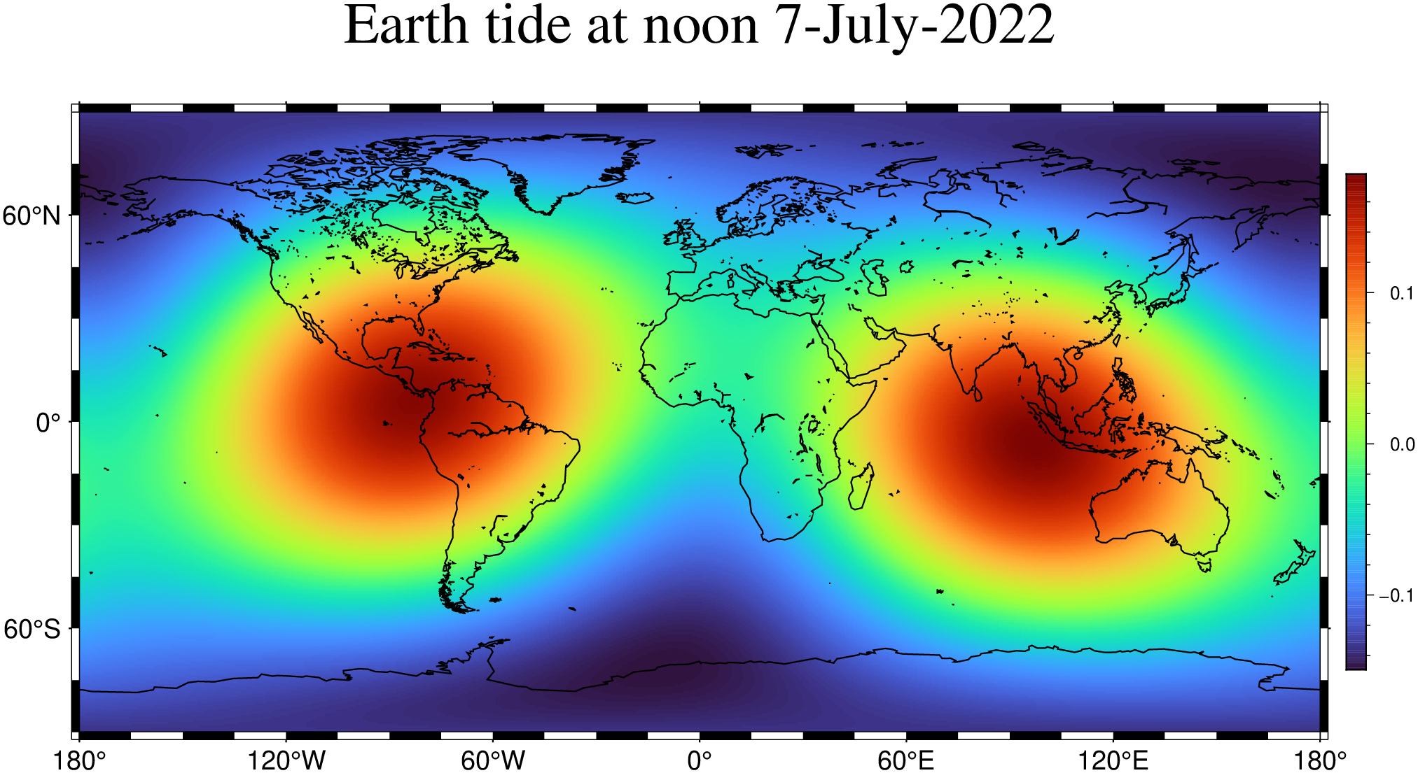
Did you know that it’s not only the oceans that have a tide? Yes, the solid Earth has tides as well, and they are not so small as one might imagine.
This example shows a global view of the vertical component of the Earth tide for a perticular data.
using GMT
GMT.resetGMT() # hide
G = earthtide(T="2022-07-07T12:00:00");
imshow(G, coast=true, colorbar=true, title="Earth tide at noon 7-July-2022")
Now we show the three components of the Earth tide for a specific location (the Panama Cannal) and time interval (the 7’th July 2022).
First we compute the components that will come out in a with named columns. This is handy because we can refer to them by name instead of by column number.
D = earthtide(range=("2022-07-07T", "2022-07-08T", "1m"), location=(-82,9))

1441×4 GMTdataset{Float64, 2}
 Row │                Time        East        North  Vertical
─────┼────────────────────────────────────────────────────────
   1 │ 2022-07-07T00:00:00  -0.0186548  -0.0120856   0.152718
   2 │ 2022-07-07T00:01:00  -0.0187063  -0.0123039   0.152364
   3 │ 2022-07-07T00:02:00  -0.0187575  -0.0125214   0.152003
   4 │ 2022-07-07T00:03:00  -0.0188083  -0.0127382   0.151636
   5 │ 2022-07-07T00:04:00  -0.0188586  -0.0129542   0.151263
   6 │ 2022-07-07T00:05:00  -0.0189085  -0.0131695   0.150883
   7 │ 2022-07-07T00:06:00  -0.018958   -0.0133839   0.150496
   8 │ 2022-07-07T00:07:00  -0.0190071  -0.0135975   0.150103
   9 │ 2022-07-07T00:08:00  -0.0190558  -0.0138102   0.149704
  10 │ 2022-07-07T00:09:00  -0.0191041  -0.0140221   0.149298
  11 │ 2022-07-07T00:10:00  -0.0191519  -0.0142331   0.148886
  12 │ 2022-07-07T00:11:00  -0.0191993  -0.0144432   0.148468
  13 │ 2022-07-07T00:12:00  -0.0192463  -0.0146525   0.148044
  ⋮  │          ⋮               ⋮            ⋮          ⋮
Now plot the three of them with a legend
D = earthtide(range="2022-07-07T/2022-07-08T/1m", location=(-82,9));    # hide
plot(D[:Time, :Vertical], lc=:red, lw=1, legend=:Vertical,
     title="Earth tide components (m) at Panama Cannal")
plot!(D[:Time, :East],  lc=:green, lw=1, legend=:East)
plot!(D[:Time, :North], lc=:blue,  lw=1, legend=:North, show=true)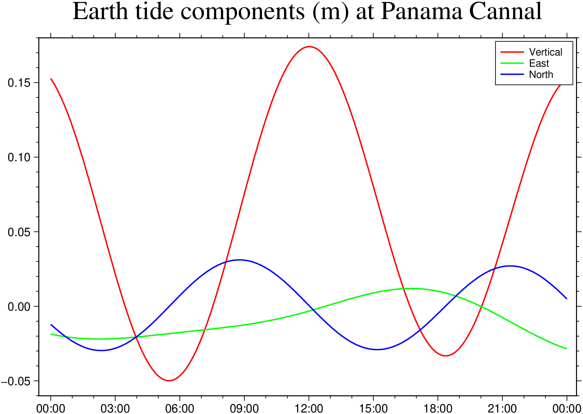
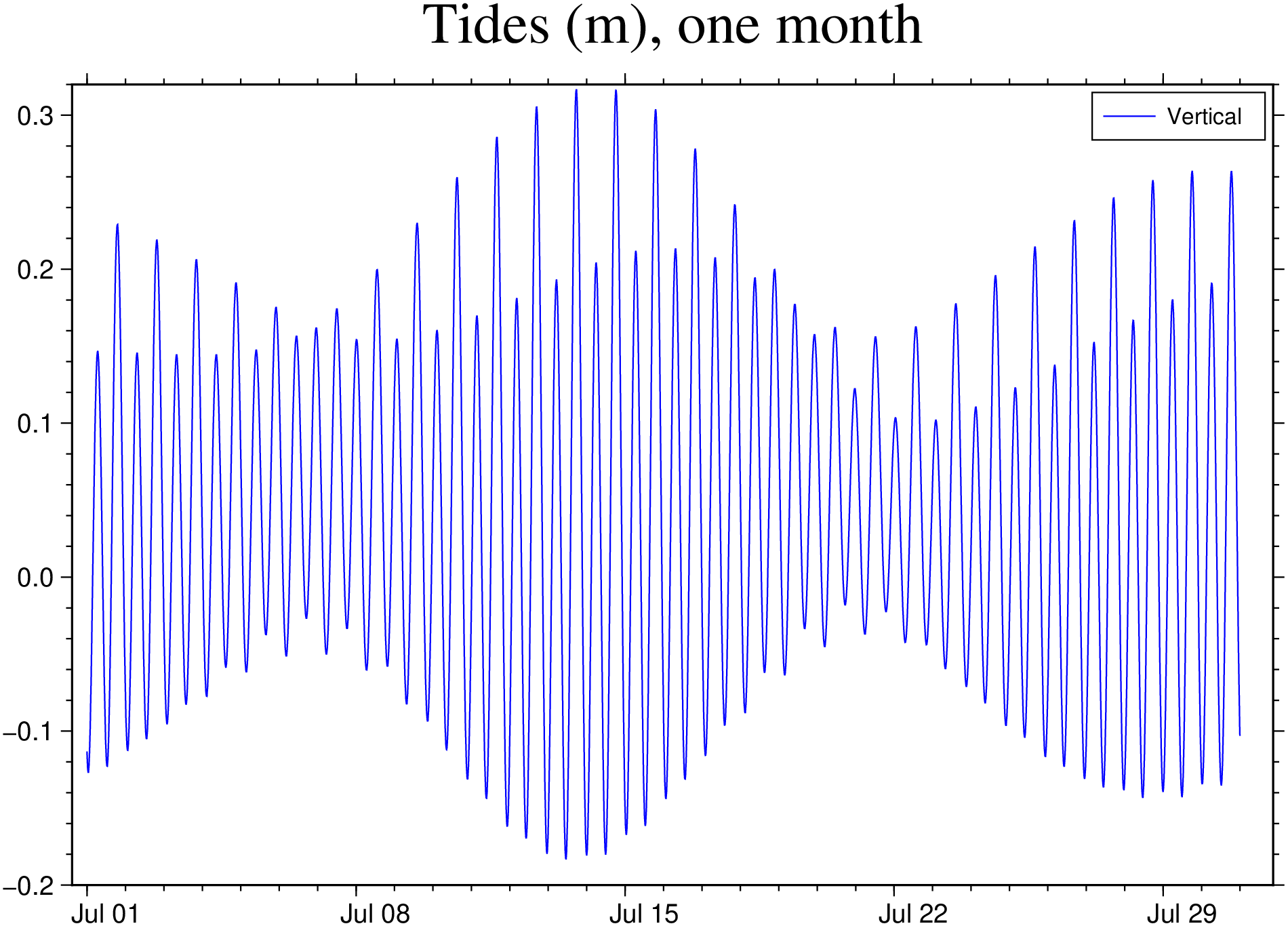
And now, let’s see a full month of tidal data (vertical component).
D = earthtide(range=("2022-07-01T", "2022-07-31T", "1m"), location=(-82,9));
plot(D[:Time, :Vertical], lc=:blue, legend=:Vertical, title="Tides (m), one month", show=true)