using GMT
gmtset(FONT_HEADING="40p,Times-Italic",)
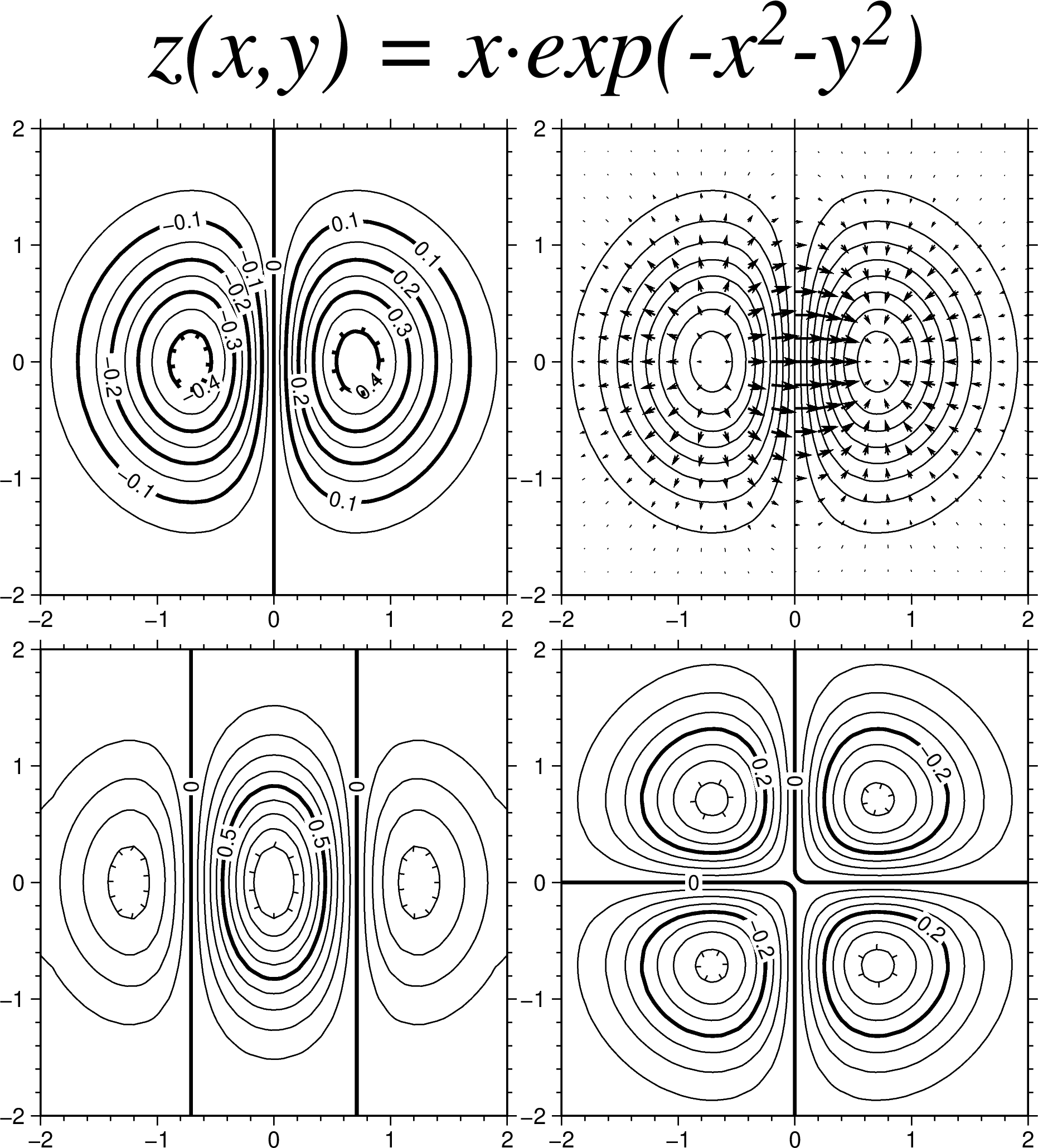
Gz = gmt("grdmath -R-2/2/-2/2 -I0.1 X Y R2 NEG EXP X MUL =");
Gdzdx = gmt("grdmath ? DDX", Gz);
Gdzdy = gmt("grdmath ? DDY", Gz);
subplot(grid=(2,2), splot_size=15, margins=0.1, title="z(x,y) = x@~\327@~exp(-x@+2@+-y@+2@+)")
grdcontour(Gz, cont=0.05, annot=0.1, labels=(dist=5,), smooth=4, ticks=(gap=(0.25,0.08),))
subplot(:set, panel=(1,2))
grdcontour(Gz, cont=0.05, labels=(dist=5,), smooth=4)
grdvector(Gdzdx, Gdzdy, inc=0.2, arrow=(len=0.25, shape=0.5, stop=true, norm=0.6),
fill=:black, pen=1, vec_scale=2)
subplot(:set, panel=(2,1))
grdcontour(Gdzdx, cont=0.1, annot=0.5, labels=(dist=5,), smooth=4, ticks=(gap=(0.25,0.08),))
subplot(:set, panel=(2,2))
grdcontour(Gdzdy, cont=0.05, annot=0.2, labels=(dist=5,), smooth=4, ticks=(gap=(0.25,0.08),))
subplot("show")