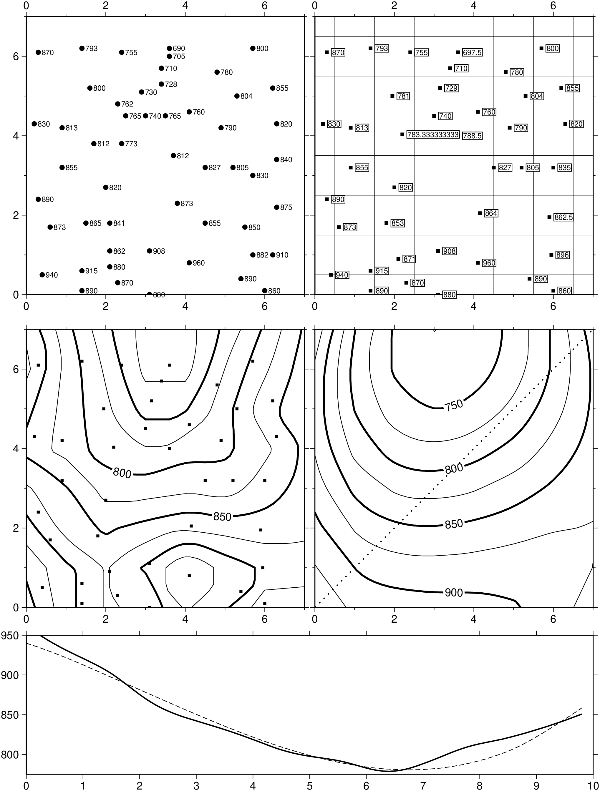
using GMT

plot("@Table_5_11.txt", limits=(0,7,0,7), frame=(axes=:WSNe, annot=2, ticks=1),
     marker=:circle, ms=0.15, fill=:black, figsize=(8,8), yshift=17)
text!("@Table_5_11.txt", offset=(0.1,0), font=6,  justify=:LM, noclip=true)
mean_xyz = blockmean("@Table_5_11.txt", region=(0,7,0,7), inc=1);

# Then draw gmt blockmean cells
basemap!(region=(0.5,7.5,0.5,7.5), frame=(grid=1,), xshift=8.3)
plot!(mean_xyz, limits=(0,7,0,7), frame=(axes=:eSNw, annot=2, ticks=1),
      marker=:square, ms=0.15, fill=:black)
# Label data values using one decimal
text!(mean_xyz, font=6, justify=:LM, zvalues="%.1f", offset=(0.15,0),
      fill=:white, clearance=0.03, pen=true, noclip=true)

# Then gmt surface and contour the data
Gdata = surface(mean_xyz, limits=(0,7,0,7), inc=1, V=:q);
grdcontour!(Gdata, frame=(axes=:WSne, annot=2, ticks=1), cont=25, annot=50,
            labels=(dist=7,), smooth=4, xshift=-8.3, yshift=-9)
plot!(mean_xyz, marker=:square, ms=0.12, fill=:black)

# Fit bicubic trend to data and compare to gridded gmt surface
Gtrend = grdtrend(Gdata, N=10, T=true);
track  = project(C=(0,0), E=(7,7), G=0.1, flat_earth=true);
grdcontour!(Gtrend, frame=(axes=:wSne, annot=2, ticks=1), cont=25, annot=50,
            smooth=4, labels=(line="CT/CB",), xshift=8.3)
plot!(track, pen=(:thick, :dot))

# Sample along diagonal
data  = grdtrack(track, G=Gdata, outcols="2,3", V=:q);
trend = grdtrack(track, G=Gtrend, outcols="2,3", V=:q);
t = gmtinfo((trend, data), inc=(0.5,25));
plot!(data, limits=t.text[1][3:end], lw=:thick, xaxis=(axes=:WSne, annot=1),
      yaxis=(annot=50,), figsize=(16.3,4), xshift=-8.3, yshift=-4.8)
plot!(trend, pen=(:thinner, :dashed), show=true)