using GMT
G = GMT.peaks();
grdcontour(G, cont=1, annot=2, show=true)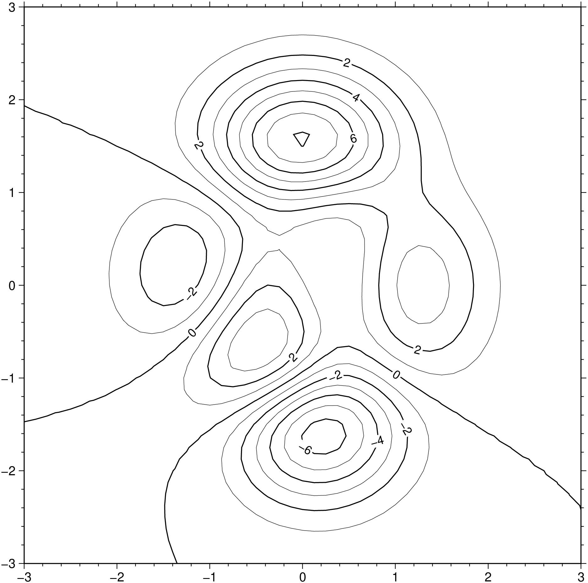
Examples created with grdcontour, contour, contourf
Contours are created with grdcontour that takes a grid as input (or a GMTgrid data type). This example shows uses the peaks function to create a classical example. Note, however, that the memory consumption in this example, when creating the plot, is much lower than traditional likewise examples because we will be using only one 2D array instead of 3 3D arrays (ref). In the example cont=1 and annot=2 means draw contours at every 1 unit of the G grid and annotate at every other contour line. axes=“a” means pick a default automatic annotation and labeling for the axes.
using GMT
G = GMT.peaks();
grdcontour(G, cont=1, annot=2, show=true)
To make colored contours we need to generate a color map and use it. Notice that we must specify a pen attribute to get the colored contours because pen specifications are always set separately. Here we will create first a colormap with makecpt that will from -6 to 8 with steps of 1. These values are picked up after the z values of the G grid.
using GMT
G = GMT.peaks();
cpt = makecpt(range=(-6,8,1));      # Create the color map
grdcontour(G, pen=(colored=true,), show=true)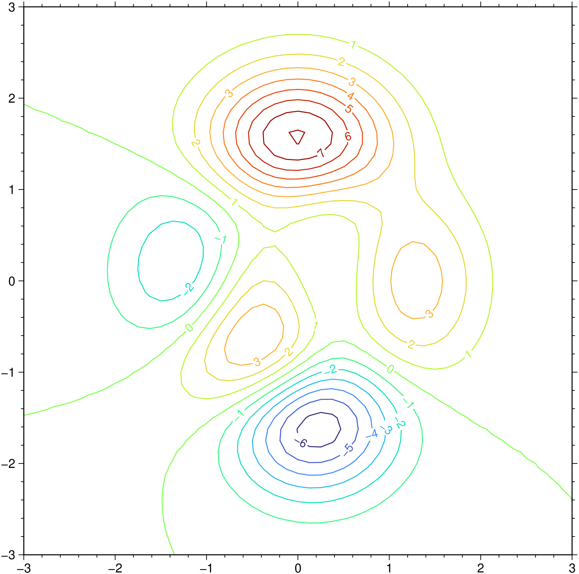
GMT does not actually have a contourf module like Matlab for example, but we can obtain the same result using grdview, grdcontour and pscontour. However, to make things the Julia wrapper wrapped up a module called contourf that makes it really easy to use. To show how it works let’s start by creating an example grid and a CPT.
using GMT
G = GMT.peaks();
C = makecpt(T=(-7,9,2));
contourf(G, C, show=true)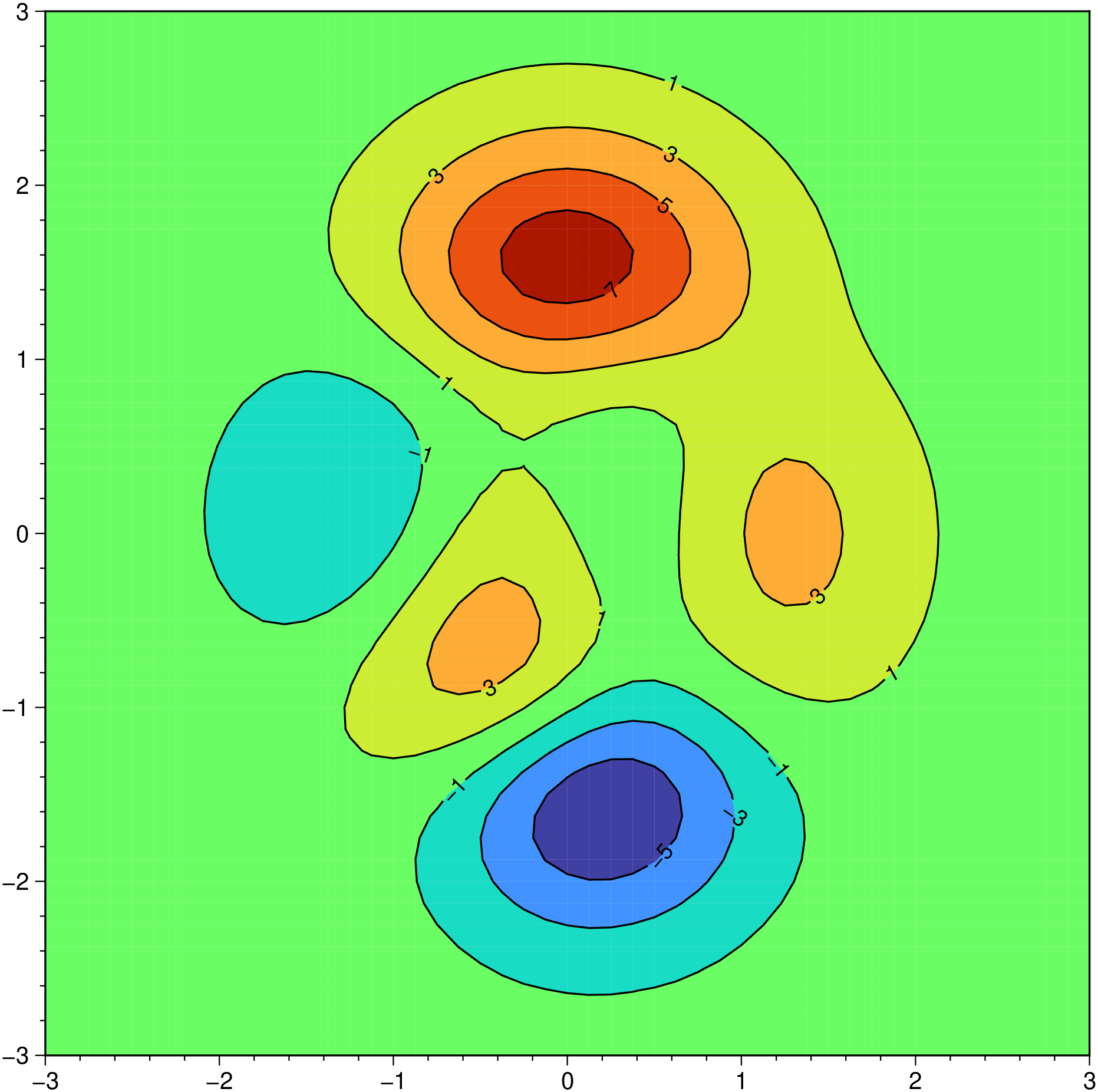
If we want to just draw some contours and not annotate them, we pass an array with the contours to be drawn.
using GMT
G = GMT.peaks();
C = makecpt(T=(-7,9,2));
contourf(G, C, contour=[-2, 0, 2, 5], show=true)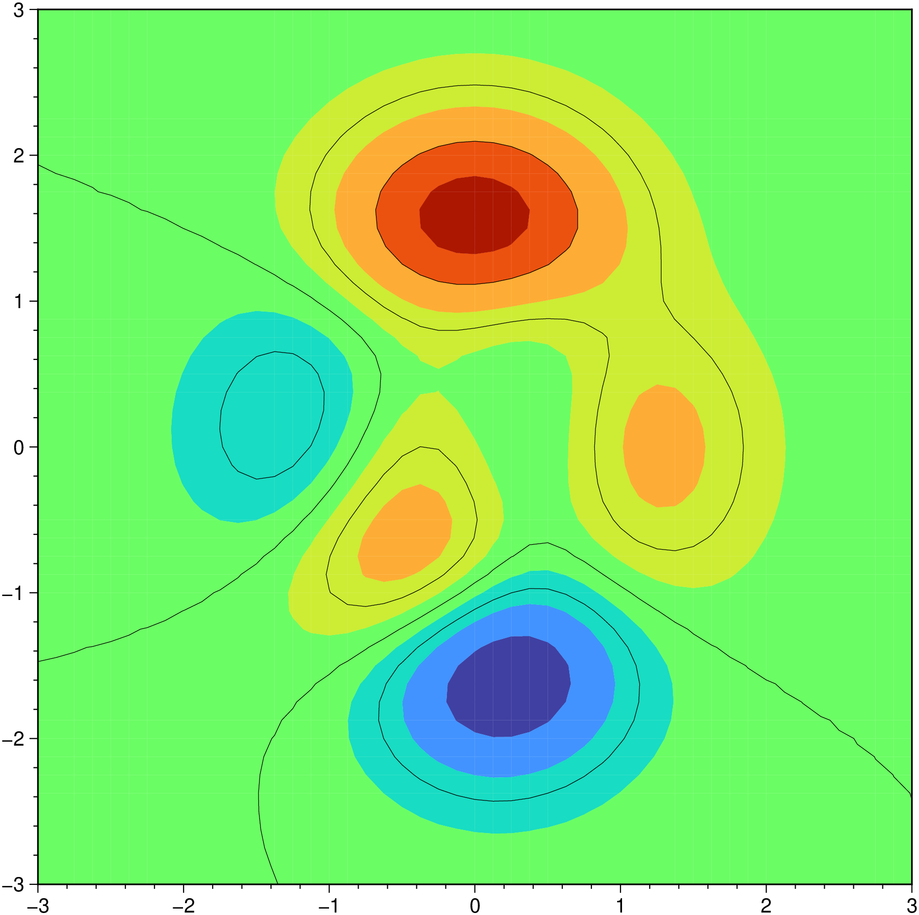
This example uses synthetic data.
using GMT
d = [0 2 5; 1 4 5; 2 0.5 5; 3 3 9; 4 4.5 5; 4.2 1.2 5; 6 3 1; 8 1 5; 9 4.5 5];
contourf(d, limits=(-0.5,9.5,0,5), pen=0.25, labels=(line=(:min,:max),), show=true)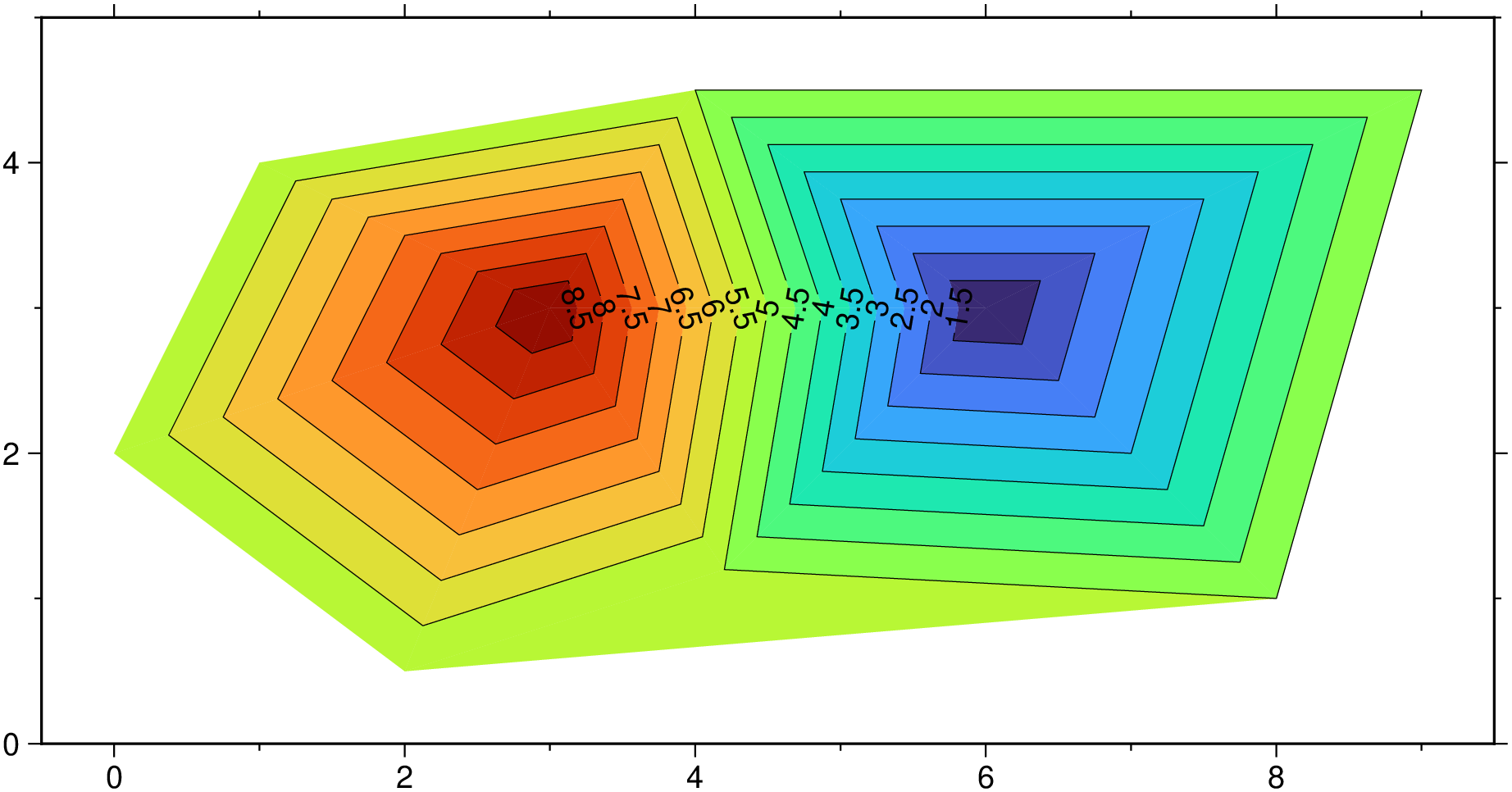
In the above since we did not specify a CPT the program picked the GMT’s default one. But if we want use another one it’s only a question of creating and passed it in.
using GMT
d = [0 2 5; 1 4 5; 2 0.5 5; 3 3 9; 4 4.5 5; 4.2 1.2 5; 6 3 1; 8 1 5; 9 4.5 5];
cpt = makecpt(range=(0,10,1), cmap=:batlow);
contourf(d, contours=cpt, limits=(-0.5,9.5,0,5), pen=0.25, labels=(line=(:min,:max),), show=true)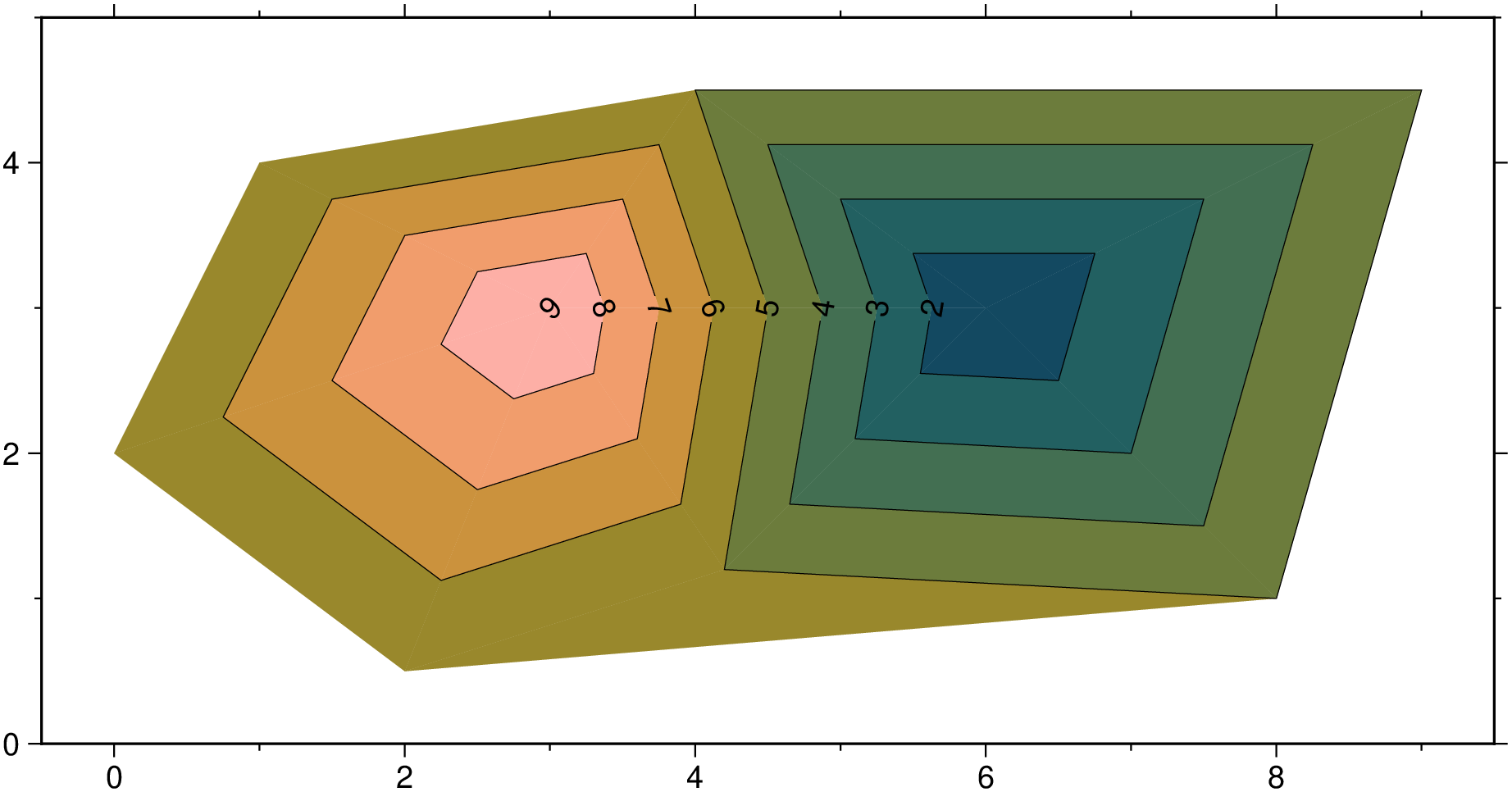
Creating a periodic 0/360 grid then selecting a central meridian for a contour map.
using GMT
G = grdmath("-Rg -I5 35 21 SDIST");    # Example grid
grdcontour(G, region=:global360, proj=(name=:Mollweide, center=35),
           cont=2000, pen=:thin, frame=:bare, coast=true, show=true)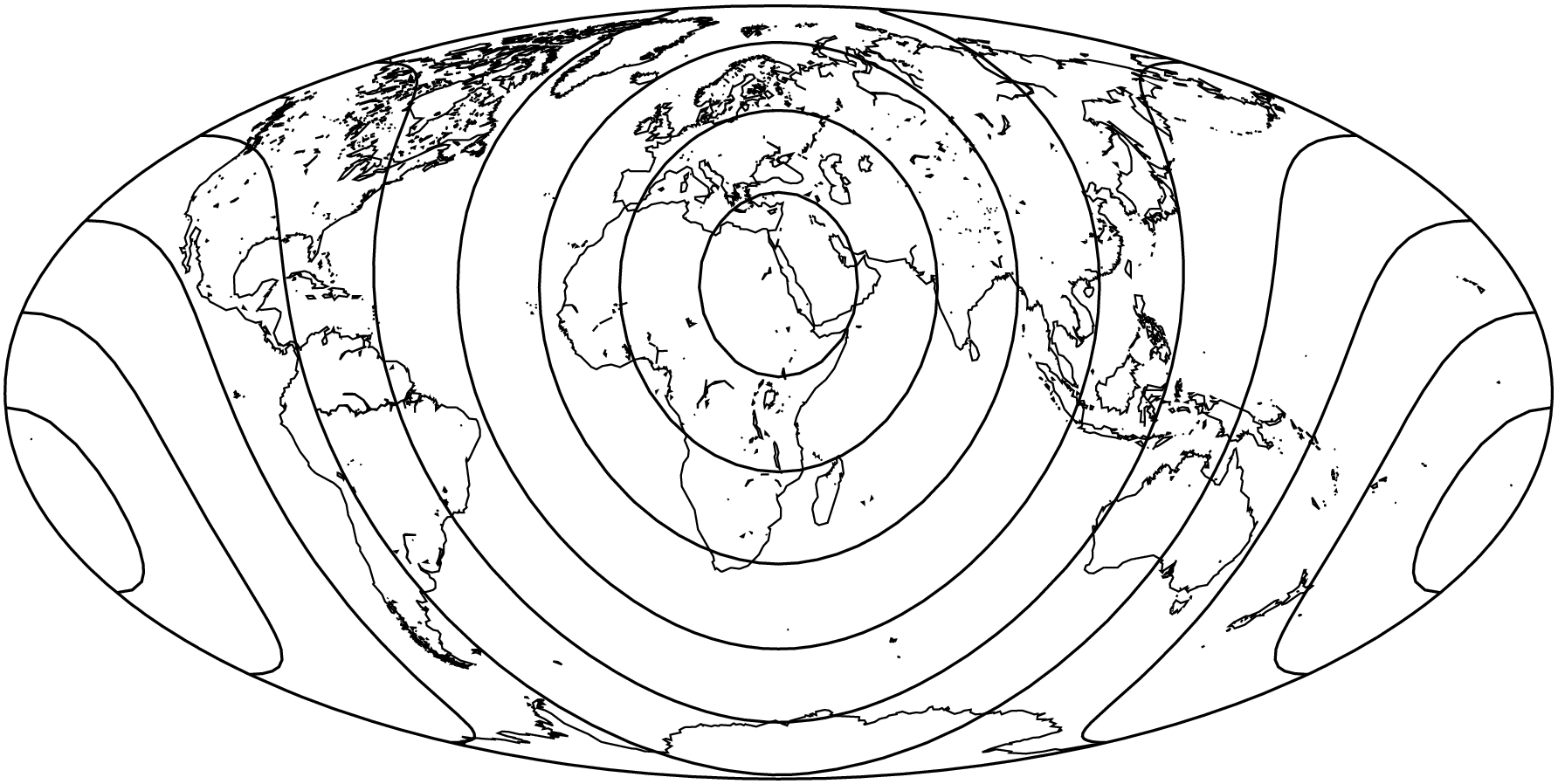
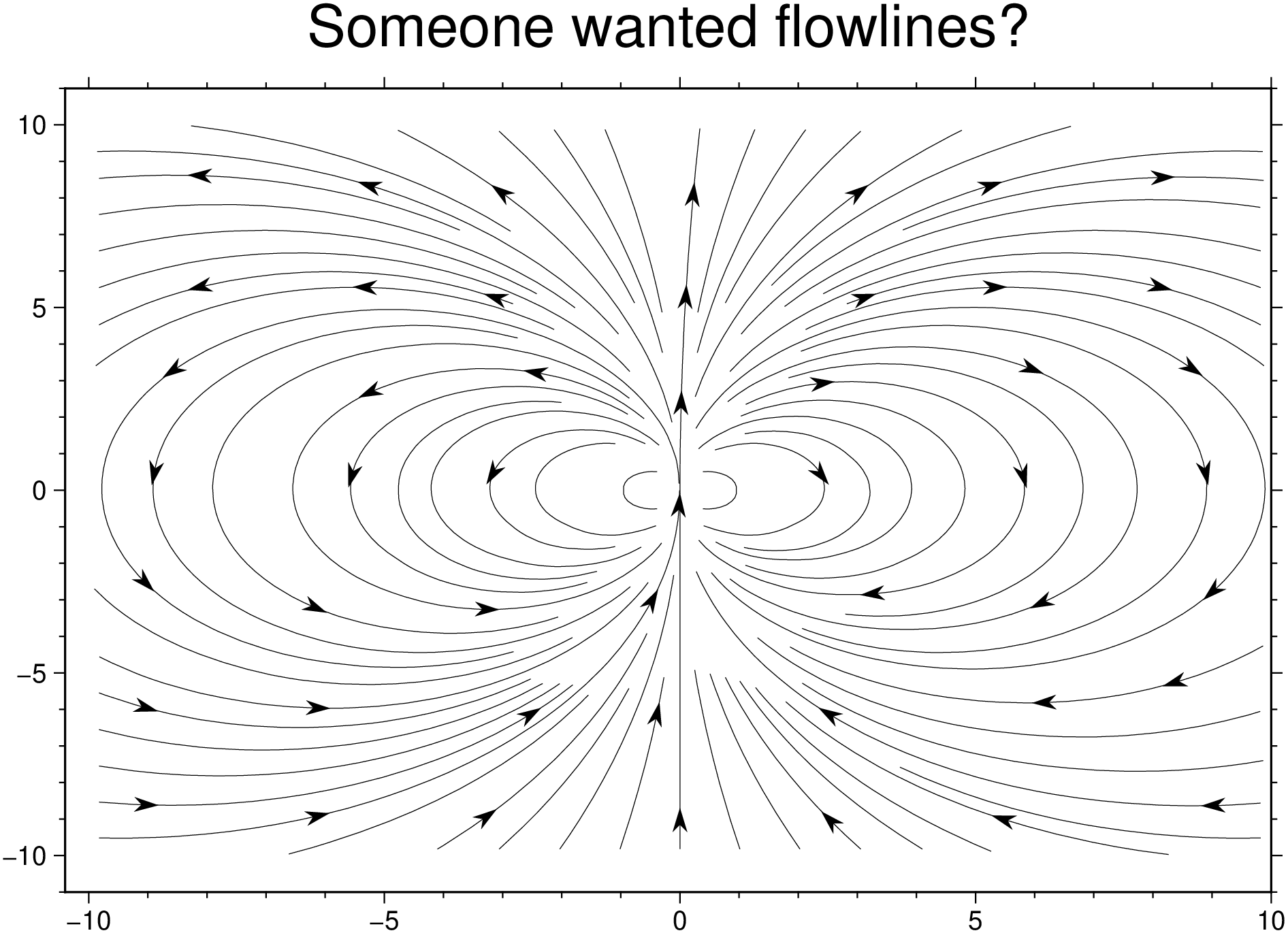
using GMT
x,y = GMT.meshgrid(-10:10);
u = 2 .* x .* y;
v = y .^2 - x .^ 2;
U = mat2grid(u, x[1,:], y[:,1]);
V = mat2grid(v, x[1,:], y[:,1]);
r,a = streamlines(U, V);
plot(r, decorated=(locations=a, symbol=(custom="arrow", size=0.3), fill=:black,
          dec2=true), title="Someone wanted flowlines?", show=true)