greenspline

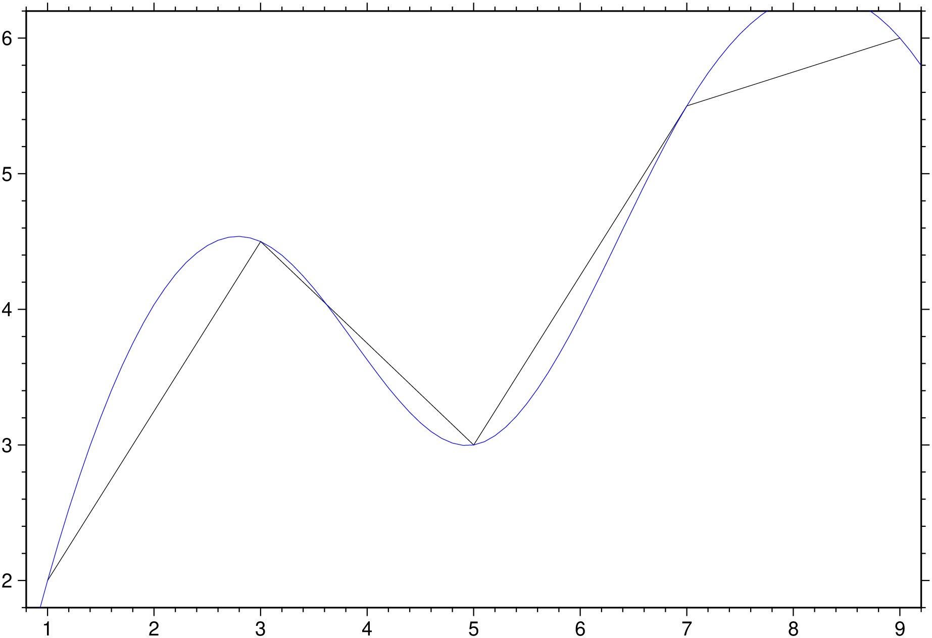
Interpolate using Green's functions for splines in 1-3 dimensions

(Warning: Manual translate by Claude. Needs revision)

Synopsis

Description

greenspline uses the Green's function for the chosen spline and geometry to interpolate data at regular or arbitrary output locations. Choose between minimum curvature, regularized, or continuous curvature splines in tension for either 1-D, 2-D, or 3-D Cartesian coordinates or spherical surface coordinates. Mathematically, the solution is composed as a sum of Green's functions and a trend function. The unknown coefficients are determined by requiring the solution to fit the observed data points exactly or approximately (via SVD).

Required Arguments

table
The name of one or more data files (or a GMTdataset or Matrix) holding the x, w data points. If no input is given then standard input is read.

Optional Arguments

A or gradient : – gradient=gradfile | gradient="gradfile+f1"
Append name of file with surface gradients to partly constrain the solution. Use modifier +f to select one of these input formats:
- 0: For 1-D data, gradient magnitude (slope) only: x, v
- 1: Records contain x, y, azimuth, v (azimuth in degrees clockwise from north) [Default for 2-D]
- 2: Records contain x, y, v, azimuth
- 3: Records contain x, direction(s), v (directions counter-clockwise from horizontal)
- 4: Records contain x, gradient components (2-D or 3-D)
- 5: Records contain x, unit vector, v (2-D or 3-D)
C or approx or approximate : – approx=cutoff | approx=(n=:, mode=:r, cutoff=0.01, file="eigen.txt", cumulative=true, incremental=true, dryrun=true)
Find an approximate surface fit using singular value decomposition (SVD) and eliminate contribution from smaller eigenvalues [Default uses Gauss-Jordan elimination for exact fit]. Append a directive:
- n: Retain only the specified number of largest eigenvalues (e.g., C=(n=100,))
- r: Retain eigenvalues whose ratio to largest eigenvalue is less than value [Default]
- v: Retain eigenvalues needed to ensure model prediction variance fraction is at least value
Optional modifiers (use as named tuple members):
- cumulative=true: Produce cumulative sum of contributions, one grid per eigenvalue (2-D only)
- incremental=true: Produce incremental sum of contributions, one grid per eigenvalue (2-D only)
- file="filename": Save eigenvalues to specified file
- dryrun=true: Save eigenvalues and exit without surface output (requires file)
D or meta or metadata: – meta=(xname="...", yname="...", zname="...", vname="...", ...)
Control netCDF grid metadata. Use named tuple with these optional members:
- xname, yname, zname: Dimension names (with optional units in brackets)
- vname: Variable name for data
- scale, offset: Scale factor and offset for data values
- invalid: Value used for NaN or missing data
- title, remark: Title and remark strings
E or misfit : – misfit=true | misfit="misfitfile" | misfit=(misfitfile="...", reportfile="...")
Evaluate spline exactly at input data locations and report misfit statistics. If E=true, statistics are written to stderr. If a filename is given, write data table augmented by spline estimate and misfit columns. If C is used with history modifiers, write eigenvalue analysis table instead. Use named tuple for multiple outputs:

E=(misfitfile="misfit.txt", reportfile="report.txt")

G or outgrid or save : – save="outfile.grd" | save="table.txt"
Specify output filename. For 2-D grids, a grid file is required. For 3-D, can be a cube file, a template for multiple 2-D grids (with floating-point format like "layer_%g.grd"), or omitted for ASCII/binary table output. For arbitrary output locations (with N), this specifies the output table name. Ignored if C is specified.
I or inc or increment or spacing : – inc=xinc | inc=(xinc,yinc) | inc=(xinc,yinc,zinc)
Specify equidistant sampling intervals. For 1-D, give xinc; for 2-D, give xinc and yinc; for 3-D, give xinc, yinc, and zinc.
L or leave_trend : – leave_trend=true | leave_trend=:t | leave_trend=:r | leave_trend=:tr
Control detrending and normalization of data prior to solving. Append directives:
- :t: Remove and restore linear least-squares trend
- :r: Normalize and restore data by maximum absolute residual value
Default applies both detrending and normalization when geometrically permissible.
N or nodes : – nodes="nodefile"
ASCII file with coordinates of desired output locations in the first column(s). The resulting values are appended to each record and written to the file given in G (or stdout).
Q or dir_derivative : – dir_derivative=az | dir_derivative=(x,y,z)
Take directional derivative instead of evaluating solution. For 1-D, give nothing (uses derivative). For 2-D, give azimuth in degrees. For 3-D, give three components of desired vector direction as a tuple; the vector will be normalized.

R or region or limits : – limits=(xmin, xmax, ymin, ymax) | limits=(BB=(xmin, xmax, ymin, ymax),) | limits=(LLUR=(xmin, xmax, ymin, ymax),units="unit") | ...more
Specify the region of interest. More at limits. For perspective view view, optionally add zmin,zmax. This option may be used to indicate the range used for the 3-D axes. You may ask for a larger w/e/s/n region to have more room between the image and the axes.

S oe splines : – splines=:c | splines=:t | splines=(:t, tension) | splines=(:q, tension, params...)
Select spline type. Append directive for spline selection:
- :c: Minimum curvature spline (1-D, 2-D, or 3-D Cartesian)
- :l: Linear or bilinear spline (1-D or 2-D Cartesian)
- :p: Minimum curvature spline for spherical surface (Parker, 1994)
- :q: Continuous curvature spline in tension for spherical surface (Wessel & Becker, 2008); append tension
- :r: Regularized spline in tension (Mitasova & Mitas, 1993); append tension and optional scale
- :t: Continuous curvature spline in tension (Wessel & Bercovici, 1998); append tension and optional scale
For :q, optional modifiers as named tuple:
- limit: Truncation error for Legendre sum [1e-6]
- n: Number of points in spline setup 10001
Example:

S=(:t, 0.7)                           # Tension 0.7
    S=(:r, 0.95, 50)                      # Tension 0.95, scale 50
    S=(:q, 0.85, limit=1e-8, n=15001)     # Spherical with custom parameters

T or mask : – mask="maskgrid"
For 2-D interpolation only. Evaluate solution only at nodes in maskgrid that are not NaN. This option eliminates the need for R, I, and r.

V or verbose : – verbose=true | verbose=level
Select verbosity level. More at verbose

W or uncertainties : – uncertainties=true | uncertainties=:w
Data one-sigma uncertainties are in the last column. Compute weights inversely proportional to uncertainties squared. Append :w if weights are given directly instead of uncertainties (no squaring). Results in weighted least squares fit. Only has effect with C.
Z or mode or distmode : – distmode=mode
Set distance mode for calculating distances between data points:
- 0: (x) in user units, Cartesian distances (1-D)
- 1: (x,y) in user units, Cartesian distances (2-D)
- 2: (x,y) in degrees, Flat Earth distances (2-D)
- 3: (x,y) in degrees, Spherical distances in km (2-D)
- 4: (x,y) in degrees, cosine of great circle arcs (spherical surface; requires S=:p or S=:q)
- 5: (x,y,z) in user units, Cartesian distances (3-D)

bi or binary_in : – binary_in=??
Select native binary format for primary table input. More at

di or nodata_in : – nodata_in=??
Substitute specific values with NaN. More at

e or pattern : – pattern=??
Only accept ASCII data records that contain the specified pattern. More at

f or colinfo : – colinfo=??
Specify the data types of input and/or output columns (time or geographical data). More at

h or header : – header=??
Specify that input and/or output file(s) have n header records. More at

i or incol or incols : – incol=col_num | incol="opts"
Select input columns and transformations (0 is first column, t is trailing text, append word to read one word only). More at incol

o or outcol : – outcol=??
Select specific data columns for primary output, in arbitrary order. More at

// Couldn't find a file when trying to resolve an input request with relative path: `common_opts/opt_r`. //

// Couldn't find a file when trying to resolve an input request with relative path: `common_opts/opt_x`. //

yx : – yx=true
Swap 1st and 2nd column on input and/or output. More at

Examples

1-D Spline

Resample 1-D data using minimum curvature spline:

using GMT

# Create sample data
data = [1.0 2.0; 3.0 4.5; 5.0 3.0; 7.0 5.5; 9.0 6.0]

# Minimum curvature spline
result = greenspline(data, region=(0,10), inc=0.1, S=:c)

Spline in tension (tension = 0.7):

result = greenspline(data, region=(0,10), inc=0.1, S=(:t, 0.7))

2-D Cartesian Grid

Create uniform grid using minimum curvature spline:

# Load data
data = gmtread("@Table_5_11.txt")

# Minimum curvature spline
G = greenspline(data, region=(0,6.5,-0.2,6.5), inc=0.1, S=:c, Z=1, save="output.nc")

Spline in tension with mask:

# Only evaluate where mask is not NaN
G = greenspline(data, T="mask.nc", S=(:t, 0.5), Z=1, save="result.nc")

Regularized spline in tension:

# Return directional derivative (NW direction, -45°)
G = greenspline(data, region=(0,6.5,-0.2,6.5), inc=0.1, S=(:r, 0.95), 
                Z=1, Q=-45, save="slopes.nc")

Approximate Fit with SVD

Cartesian cubic spline retaining 100 largest eigenvalues:

G = greenspline(data, region=(0,6.5,-0.2,6.5), inc=0.1, S=:c, Z=1, 
                C=(n=100,), save="approx.nc")

Evaluate cumulative contributions:

# Creates files contribution_cum_000.nc, contribution_cum_001.nc, etc.
greenspline(data, region=(0,6.5,-0.2,6.5), inc=0.1, S=:c, Z=1,
            C=(cumulative=true,), save="contribution.nc")

Surface with Gradient Constraints

Recover surface from single point value and gradient constraints:

# Point data in pt.txt, gradients in slopes.txt  
G = greenspline("pt.txt", region=(-3.2,3.2,-3.2,3.2), inc=0.1, S=:c, Z=1,
                A="slopes.txt+f1", save="surface.nc")

3-D Cartesian Interpolation

Create 3-D grid from (x,y,z,w) data:

# ASCII table output
result = greenspline("@Table_5_23.txt", region=(5,40,-5,10,5,16), 
                     inc=0.25, S=(:r, 0.85), Z=5)

# Multiple 2-D layer grids
greenspline("@Table_5_23.txt", region=(5,40,-5,10,5,16), inc=0.25,
            S=(:r, 0.85), Z=5, save="layer_%g.grd")

# Single 3-D netCDF cube
greenspline("@Table_5_23.txt", region=(5,40,-5,10,5,16), inc=0.25,
            S=(:r, 0.85), Z=5, save="cube3d.nc")

Spherical Surface Interpolation

Global grid using Parker spline:

# Minimum curvature on sphere
G = greenspline("@mag_obs_1990.txt", region=:global, inc=1, S=:p, Z=3);

With tension:

# Continuous curvature in tension (tension = 0.85)
G = greenspline("@mag_obs_1990.txt", region=:global, inc=1, S=(:q, 0.85), Z=3)

Arbitrary Output Locations

Output at specific coordinates:

# Nodes specified in nodefile.txt
greenspline(data, N="nodefile.txt", S=:c, Z=1, save="output.txt")

Misfit Evaluation

Evaluate fit quality:

# Statistics to stderr
greenspline(data, region=(0,6.5,-0.2,6.5), inc=0.1, S=:c, Z=1, 
            E=true, save="grid.nc")

# Write augmented data table with estimates and misfits
greenspline(data, region=(0,6.5,-0.2,6.5), inc=0.1, S=:c, Z=1,
            E="misfits.txt", save="grid.nc")

Notes

Memory Requirements

The solution requires inverting an n × n double precision matrix, where n is the number of data constraints. Memory usage scales as n²:

n = 1,024: ~8 MB
n = 10,240: ~800 MB

Pre-process data with blockmean, blockmedian, or blockmode to avoid aliasing and control n. For spherical data, use gmtspatial nearest neighbor reduction.

Boundary Conditions

For Cartesian cases, free-space Green functions are used, so no boundary conditions apply at domain edges. For specific boundary conditions, consider using surface instead.

Numerical Stability

The inversion can become unstable when data neighbors are very close compared to the overall data span. Remedies:

Pre-process data by averaging closely spaced neighbors
Use SVD solution (C) and discard smallest eigenvalues

Tension Parameter

Tension suppresses spurious oscillations from minimum curvature requirement, especially with rapid gradient changes:

Smooth data (e.g., potential fields): Little or no tension needed
Rough data (e.g., topography): Moderate tension typically better

Experiment with a range of values. For regularized spline (S=:r), the scale value has limited stable range—experiment to find valid settings.

1-D Splines

Unlike sample1d (which offers traditional splines with standard boundary conditions like natural cubic spline), greenspline's 1-D spline does not specify boundary conditions at domain ends.

Eigenvalue Selection

For approximate fits (C), it may be difficult to determine how many eigenvalues to retain. The cumulative and incremental modifiers create solutions for all cutoff selections, allowing animation to explore changes and select appropriate C values. See GMT animations for examples.

Spherical Splines

The series solution for S=:q (Wessel & Becker, 2008) is slower to compute, so values are pre-calculated and cubic spline interpolation lookup is used. Optional modifiers limit and n control accuracy and performance.

References

Davis, J. C., 1986, Statistics and Data Analysis in Geology, 2nd Edition, 646 pp., Wiley, New York.
Mitasova, H., and L. Mitas, 1993, Interpolation by regularized spline with tension: I. Theory and implementation, Math. Geol., 25, 641-655.
Parker, R. L., 1994, Geophysical Inverse Theory, 386 pp., Princeton Univ. Press, Princeton, N.J.
Sandwell, D. T., 1987, Biharmonic spline interpolation of Geos-3 and Seasat altimeter data, Geophys. Res. Lett., 14, 139-142.
Wessel, P., and D. Bercovici, 1998, Interpolation with splines in tension: a Green's function approach, Math. Geol., 30, 77-93, https://doi.org/10.1023/A:1021713421882.
Wessel, P., and J. M. Becker, 2008, Interpolation using a generalized Green's function for a spherical surface spline in tension, Geophys. J. Int, 174, 21-28, https://doi.org/10.1111/j.1365-246X.2008.03829.x.
Wessel, P., 2009, A general-purpose Green's function interpolator, Computers & Geosciences, 35, 1247-1254, https://doi.org/10.1016/j.cageo.2008.08.012.

Navigation