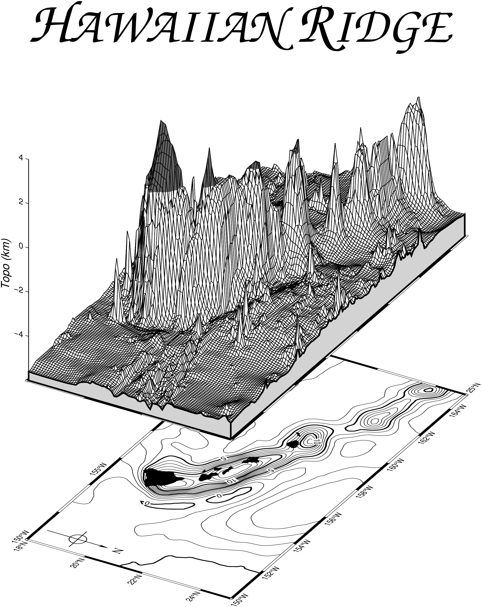
(4) A 3-D perspective mesh plot

This example will illustrate how to make a fairly complicated composite figure. We need a subset of the ETOPO5 bathymetry 1 and Geosat geoid data sets which we have extracted from the global data grids using grdcut and access those files here as remote files on the GMT data server. We would like to show a 2-layer perspective plot where layer one shows a contour map of the marine geoid with the location of the Hawaiian islands superposed, and a second layer showing the 3-D mesh plot of the topography. We also add an arrow pointing north and some text. The first part of this script shows how to do it:

using GMT

makecpt(cmap=(255,100), range=(-10,10,10), no_bg=true);
grdcontour("@HI_geoid_04.nc", region=(195,210,18,25), view=(60,30), cont=1,
           annot=(int=5, labels=(rounded=true,)), labels=(dist=10,),
           xshift=3, yshift=3, proj=:merc, figscale=1.1)
coast!(p=true, frame=(annot=2, axes=:NEsw), land=:black,
       rose=(inside=true, anchor=:BR, width=2.5, offset=0.25, label=true))
grdview!("@HI_topo_04.nc", p=true, region=(195,210,18,25,-6,4),
         plane=(-6,:lightgray), surftype=(surf=true, mesh=true), Jz="0.9",
         frame=(axes=:wesnZ, annot=2), zaxis=(annot=2, label="Topo (km)"), yshift=5.6)
text!("H@#awaiian@# R@#idge@#", x=7.5, y=14.0, region=(0,21,0,28),
      font=(60,"ZapfChancery-MediumItalic"), justify=:CB, proj=:linear,
      view=:none, figscale=1, show=true)

The purpose of the CPT zero.cpt is to have the positive topography mesh painted light gray (the remainder is white). The left side of Figure shows the complete illustration.

The second part of the script shows how to make the color version of this figure that was printed in our first article in EOS Trans. AGU (8 October 1991). Using grdview one can choose to either plot a mesh surface (left) or a color-coded surface (right). We have also added artificial illumination from a light-source due north, which is simulated by computing the gradient of the surface grid in that direction though the grdgradient program. We choose to use the -Qc option in grdview to achieve a high degree of smoothness. Here, we select 100 dpi since that will be the resolution of our final raster (The EOS raster was 300 dpi). Note that the size of the resulting output file is directly dependent on the square of the dpi chosen for the scanline conversion and how well the resulting image compresses. A higher value for dpi in -Qc would have resulted in a much larger output file. The CPTs were taken from Example (2) Image presentations.