contour

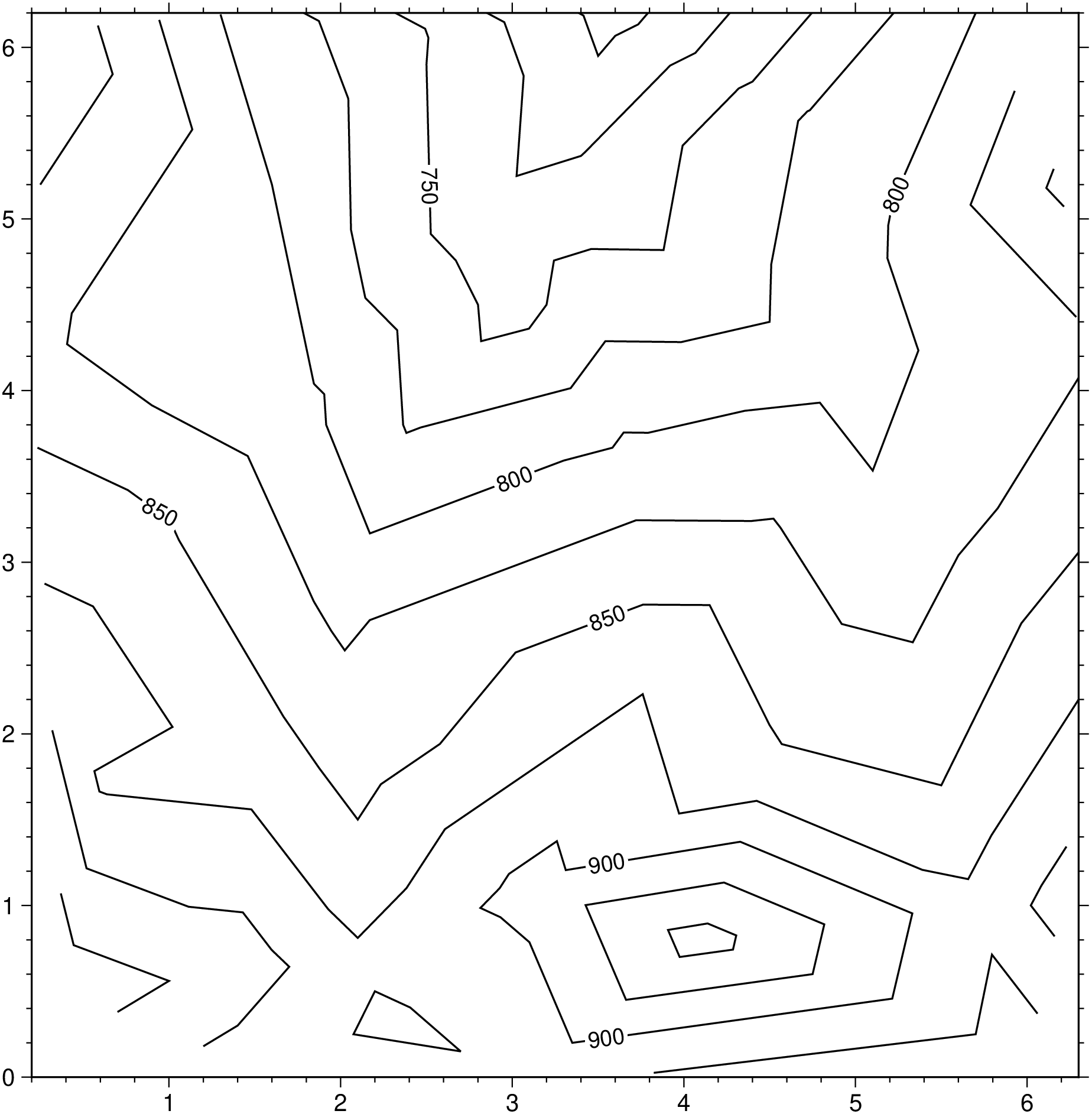
contour(cmd0::String="", arg1=nothing; kwargs...)

keywords: GMT, Julia, contour plots, mapping

Contour plot from table data by direct triangulation

Description

Reads data from file or table and produces a raw contour plot by triangulation. By default, the optimal Delaunay triangulation is performed using Shewchuk's [1996], but the user may optionally provide a second file with network information, such as a triangular mesh used for finite element modeling. In addition to contours, the area between contours may be painted according to the CPT. Alternatively, the x, y, z positions of the contour lines may be saved to one or more output files (or standard output) and no plot is produced.

Required Arguments

table
One or more data tables holding a number of data columns.

J or proj or projection : – proj=<parameters>
Select map projection. More at proj

R or region or limits : – limits=(xmin, xmax, ymin, ymax) | limits=(BB=(xmin, xmax, ymin, ymax),) | limits=(LLUR=(xmin, xmax, ymin, ymax),units="unit") | ...more
Specify the region of interest. More at limits. For perspective view view, optionally add zmin,zmax. This option may be used to indicate the range used for the 3-D axes. You may ask for a larger w/e/s/n region to have more room between the image and the axes.

Optional Arguments

A or annot or annotation : – annot=annot_int | annot=(int=annot_int, disable=true, single=true, labels=labelinfo)
annot_int is annotation interval in data units; it is ignored if contour levels are given in a file. [Default is no annotations]. Use annot=(disable=true,) to disable all annotations implied by cont. Alternatively do annot=(single=true, int=val) to plot val as a single contour. The optional labelinfo controls the specifics of the label formatting and consists of a named tuple with the following control arguments Label formatting

B or axes or frame
Set map boundary frame and axes attributes. Default is to draw and annotate left, bottom and vertical axes and just draw left and top axes. More at frame

C or cont or contours or levels : – cont=cont_int
The contours to be drawn may be specified in one of four possible ways:
1. If cont_int has the suffix ".cpt" and can be opened as a file, it is assumed to be a CPT. The color boundaries are then used as contour levels. If the CPT has annotation flags in the last column then those contours will be annotated. By default all contours are labeled; use annot=(disable=true,)) (or annot=:none) to disable all annotations.
2. If cont_int is a file but not a CPT, it is expected to contain contour levels in column 1 and a C(ontour) OR A(nnotate) in col 2. The levels marked C (or c) are contoured, while the levels marked A (or a) are contoured and annotated. If the annotation angle is present we will plot the label at that fixed angle [aligned with the contour]. Finally, a contour- specific pen may be present and will override the pen set by pen for this contour level only. Note: Please specify pen in proper format so it can be distinguished from a plain number like angle. If only cont-level columns are present then we set type to C
3. If cont_int is a constant or an array it means plot those contour intervals. This works also to draw single contours. E.g. contour=[0] will draw only the zero contour. The annot option offers the same list choice so they may be used together to plot a single annotated contour and another single non-annotated contour, as in anot=[10], cont=[5] that plots an annotated 10 contour and an non-annotated 5 contour. If annot is set and cont is not, then the contour interval is set equal to the specified annotation interval.
4. If no argument is given in modern mode then we select the current CPT.
5. Otherwise, cont_int is interpreted as a constant contour interval.
If a file is given and ticks is set, then only contours marked with upper case C or A will have tick-marks. In all cases the contour values have the same units as the grid. Finally, if neither cont nor annot are set then we auto-compute suitable contour and annotation intervals from the data range, yielding 10-20 contours.

D or dump : – dump=fname
Dump contours as data line segments; no plotting takes place. Append filename template which may contain C-format specifiers. If no filename template is given we return the result in a GMTdataset. If filename has no specifiers then we write all lines to a single file. If a float format (e.g., %6.2f) is found we substitute the contour z-value. If an integer format (e.g., %06d) is found we substitute a running segment count. If an char format (%c) is found we substitute C or O for closed and open contours. The 1-3 specifiers may be combined and appear in any order to produce the the desired number of output files (e.g., just %c gives two files, just %f would separate segments into one file.
E or index : – index="indexfile[+b]" | index=dataset
Give name of file with network information. Each record must contain triplets of node numbers for a triangle [Default computes these using Delaunay triangulation (see triangulate)]. If the indexfile is binary and can be read the same way as the binary input table then you can append +b to spead up the reading [Default reads nodes as ASCII]. index=dataset uses a already in-memory matrix or GMTdataset.
G or labels : – labels=()
The required argument controls the placement of labels along the quoted lines. Choose among five controlling algorithms as explained in Placement methods
I or fill or colorize : – fill=true
Color the triangles using the CPT.
L or mesh : – mesh=pen\ Draw the underlying triangular mesh using the specified pen attributes [Default is no mesh].
N or no_clip : – no_clip=true
Do NOT clip contours or image at the boundaries [Default will clip to fit inside region region].
Q or cut : – cut=np | cut=length&unit[+z]
Do not draw contours with less than np number of points [Draw all contours]. Alternatively, give instead a minimum contour length in distance units, including c (Cartesian distances using user coordinates) or C for plot length units in current plot units after projecting the coordinates. Optionally, append +z to exclude the zero contour.
S or skip : – skip=true | skip=:p|:t
Skip all input *xyz points that fall outside the region [Default uses all the data in the triangulation]. Alternatively, use skip=:t to skip triangles whose three vertices are all outside the region. skip=true is interpreted as skip=:p.
T or ticks : – ticks=(local_high=true, local_low=true, gap=gap, closed=true, labels=labels)
Will draw tick marks pointing in the downward direction every gap along the innermost closed contours only; set closed=true to tick all closed contours. Use gap=(gap,length) and optionally tick mark length (append units as c, i, or p) or use defaults ["15p/3p"]. User may choose to tick only local highs or local lows by specifying local_high=true, local_low=true, respectively. Set labels to annotate the centers of closed innermost contours (i.e., the local lows and highs). If no labels (i.e, set labels="") is set, we use - and + as the labels. Appending exactly two characters, e.g., labels=:LH, will plot the two characters (here, L and H) as labels. For more elaborate labels, separate the low and hight label strings with a comma (e.g., labels="lo,hi"). If a file is given by cont, and ticks is set, then only contours marked with upper case C or A will have tick marks [and annotations].

U or time_stamp : – time_stamp=true | time_stamp=(just="code", pos=(dx,dy), label="label", com=true)
Draw GMT time stamp logo on plot. More at timestamp

V or verbose : – verbose=true | verbose=level
Select verbosity level. More at verbose

W or pen=pen
Set pen attributes for the arrow stem [Defaults: width = default, color = black, style = solid]. See Pen attributes

X or xshift or x_offset : xshift=true | xshift=x-shift | xshift=(shift=x-shift, mov="a|c|f|r")
Shift plot origin. More at xshift

Y or yshift or y_offset : yshift=true | yshift=y-shift | yshift=(shift=y-shift, mov="a|c|f|r")
Shift plot origin. More at yshift

figname or savefig or name : – figname=name.png
Save the figure with the figname=name.ext where ext chooses the figure image format.

bi or binary_in : – binary_in=??
Select native binary format for primary table input. More at

bo or binary_out : – binary_out=??
Select native binary format for table output. More at

di or nodata_in : – nodata_in=??
Substitute specific values with NaN. More at

e or pattern : – pattern=??
Only accept ASCII data records that contain the specified pattern. More at

f or colinfo : – colinfo=??
Specify the data types of input and/or output columns (time or geographical data). More at

g or gap : – gap=??
Examine the spacing between consecutive data points in order to impose breaks in the line. More at

h or header : – header=??
Specify that input and/or output file(s) have n header records. More at

i or incol or incols : – incol=col_num | incol="opts"
Select input columns and transformations (0 is first column, t is trailing text, append word to read one word only). More at incol

Normally, the annotated contour is selected for the legend. You can select the regular contour instead, or both of them, by considering the label to be of the format [annotcontlabel][/contlabel]. If either label contains a slash (/) character then use | as the separator for the two labels instead. .. include:: explain-l.rst

q or inrows : – inrows=??
Select specific data rows to be read and/or written. More at

yx : – yx=true
Swap 1st and 2nd column on input and/or output. More at

p or view or perspective : – view=(azim, elev)
Default is viewpoint from an azimuth of 200 and elevation of 30 degrees.
Specify the viewpoint in terms of azimuth and elevation. The azimuth is the horizontal rotation about the z-axis as measured in degrees from the positive y-axis. That is, from North. This option is not yet fully expanded. Current alternatives are:
- view=??
  A full GMT compact string with the full set of options.
- view=(azim,elev)
  A two elements tuple with azimuth and elevation
- view=true
  To propagate the viewpoint used in a previous module (makes sense only in bar3!)
More at perspective

s or skiprows or skip_NaN : – skip_NaN=true | skip_NaN="<cols[+a][+r]>"
Suppress output of data records whose z-value(s) equal NaN. More at

t or transparency or alpha: – alpha=50
Set PDF transparency level for an overlay, in (0-100] percent range. [Default is 0, i.e., opaque]. Works only for the PDF and PNG formats.

Units

For map distance unit, append unit d for arc degree, m for arc minute, and s for arc second, or e for meter [Default unless stated otherwise], f for foot, k for km, M for statute mile, n for nautical mile, and u for US survey foot. By default we compute such distances using a spherical approximation with great circles (-jg) using the authalic radius (see PROJ_MEAN_RADIUS). You can use -jf to perform “Flat Earth” calculations (quicker but less accurate) or -je to perform exact geodesic calculations (slower but more accurate; see PROJ_GEODESIC for method used).

Examples

To make a raw contour plot from the remote file Table_5.11.txt and draw the contours every 25 and annotate every 50, using the default Cartesian projection, try

using GMT
contour("@Table_5_11.txt", pen=:thin, contour=25, annot=50, show=true)

To use the same data but only contour the values 750 and 800, use

using GMT
contour("@Table_5_11.txt", annot=[750,800], pen=0.5, show=true)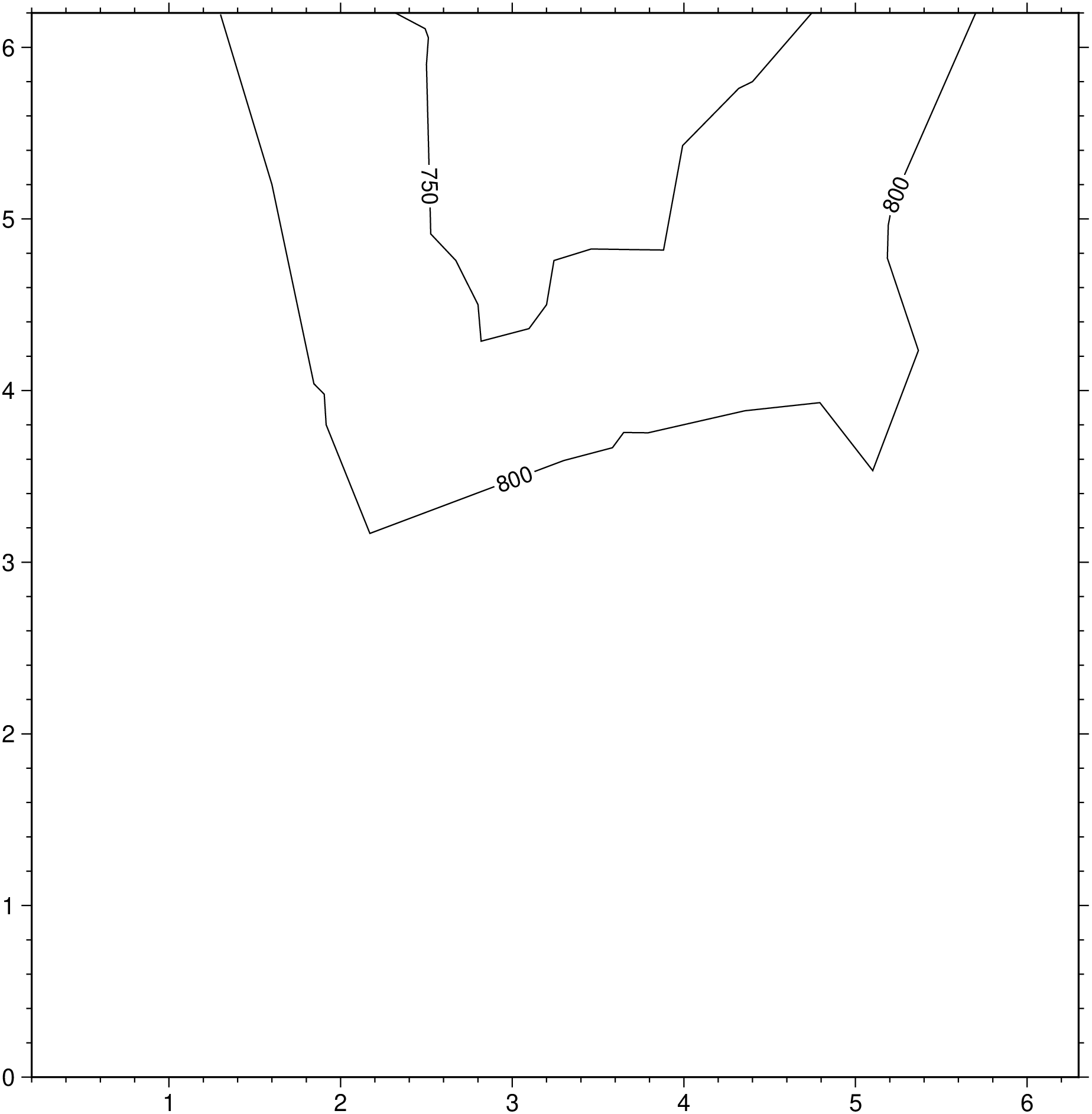

To create a color plot of the numerical temperature solution obtained on a triangular mesh whose node coordinates and temperatures are stored in temp.xyz and mesh arrangement is given by the file mesh.ijk, using the colors in temp.cpt, run

contour("temp.xyz", index="mesh.ijk", region=(0,150,0,100), figscale=0.25,
            cmap="temp.cpt", labels=true, pen=0.25, show=true)

To save the triangulated 100-m contour lines in topo.txt and separate them into multisegment files (one for each contour level), try

contour("topo.txt", contour=100, dump="contours_%.0f.txt")

References

Watson, D. F., 1982, Acord: Automatic contouring of raw data, Comp. & Geosci., 8, 97-101.

Shewchuk, J. R., 1996, Triangle: Engineering a 2D Quality Mesh Generator and Delaunay Triangulator, First Workshop on Applied Computational Geometry (Philadelphia, PA), 124-133, ACM, May 1996.

http://www.cs.cmu.edu/~quake/triangle.html

Auto-legend entries

This module allows you to use the l option to specify an automatic legend entry. This option is available for lines or symbols only. If the symbol size is variable and computed from other information (which may be true for some symbols deriving their size from other input columns), then you need to supply a representative legend size via the +S modifier.

Navigation