using GMT
coast(region=:global, proj=:Mollweide, shore=true, show=true)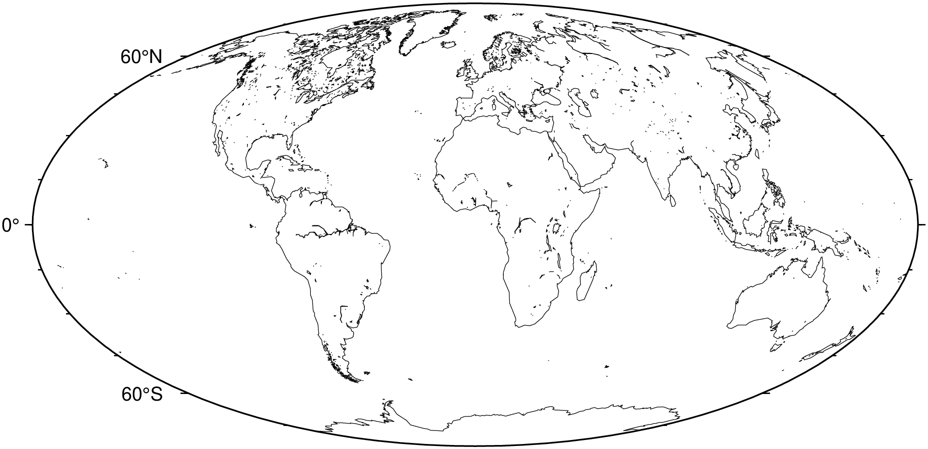
GMT uses the coast utility to access a version of the GSHHG data specially formatted for GMT. The GSHHG data have strengths and weaknesses. It is global and open source, but is based on relatively old datasets and hence may not be accurate enough for very large-scale mapping projects. For more information about the coastlines data-set see the GSHHG repository
Use the shore option to plot only the shorelines:
using GMT
coast(region=:global, proj=:Mollweide, shore=true, show=true)
The shorelines are divided in 4 levels:
You can specify which level you want to plot by appending the level number and a GMT pen configuration to the shore option. For example, to plot just the coastlines with 0.5 thickness and black lines:
using GMT
coast(region=:global, proj=:Mollweide, shore=(level=1, pen=(0.5,:black)), show=true)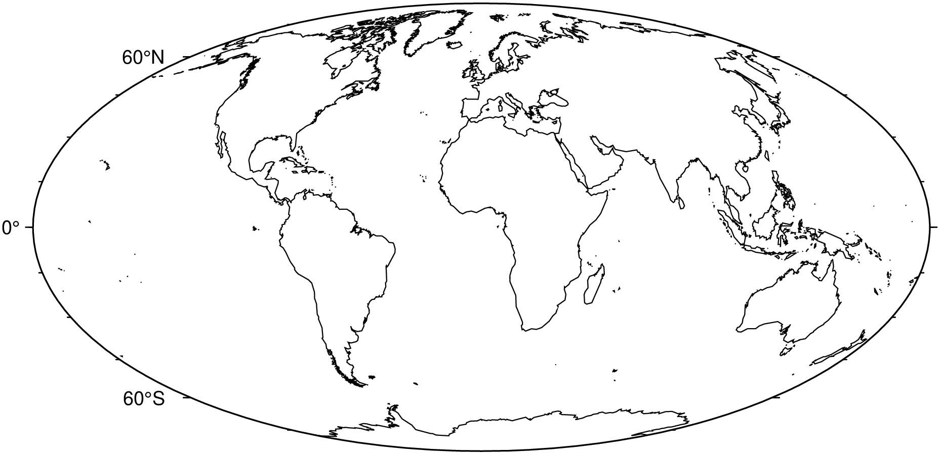
We can specify multiple levels by using the shore option more than once by using a Tuple of NamedTuples. That is, in this case we can no longer use the simpler form we used above but must instead do:
using GMT
coast(region=:global, proj=:Mollweide,
      shore=((level=1, pen=(0.5,:black)), (level=2, pen=(0.5,:red))), show=true)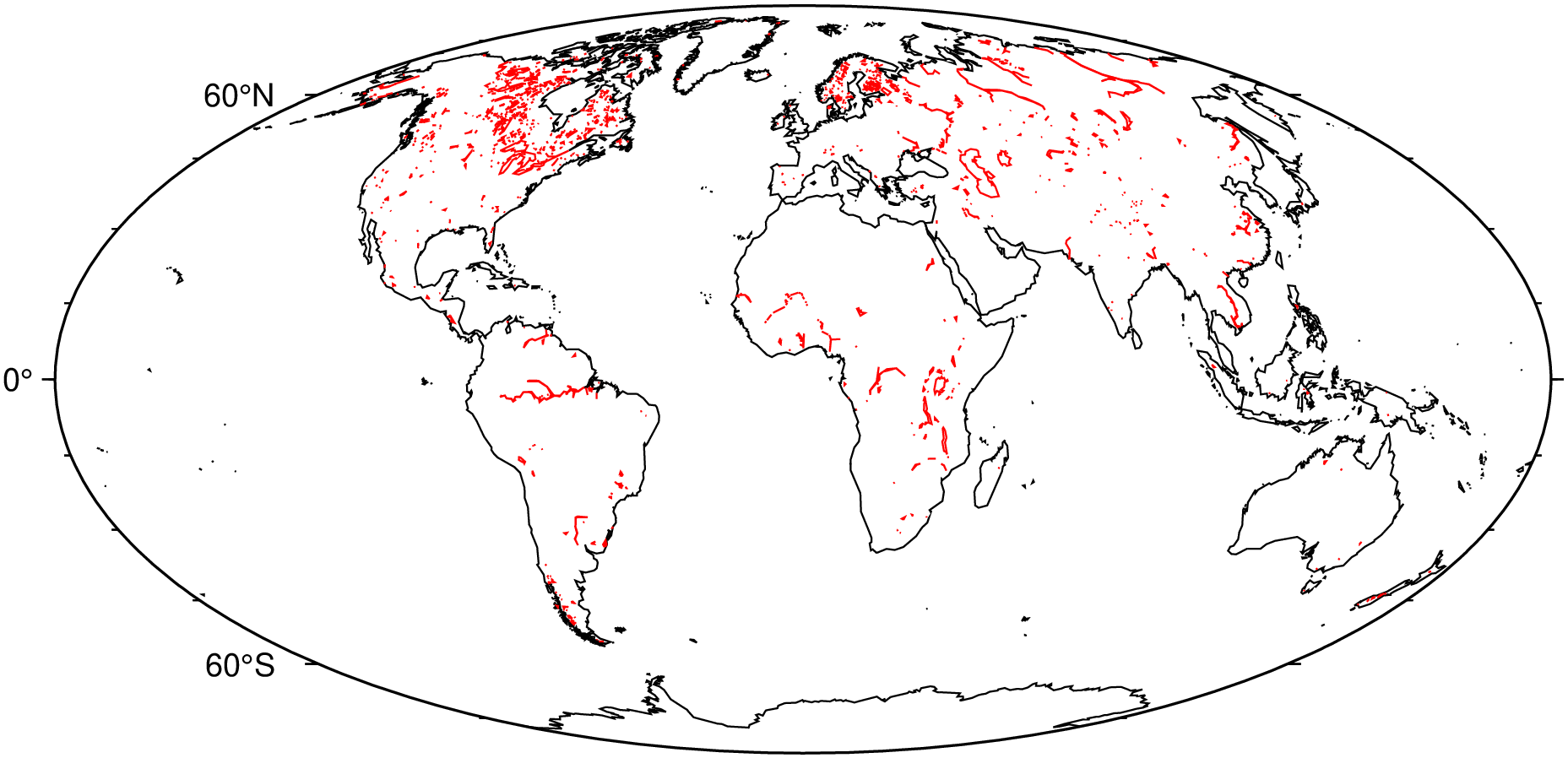
Resolutions
The coastline database comes with 5 resolutions, which can be set using the res or resolution options. The resolution drops by 80% between levels:
using GMT

# Need to take one out of the cycle to start the figure.
coast(region=(-158.3,-157.6,21.2,21.8), proj=:Mercator, res=:crude, shore=1, frame=:none)
for res in ["low", "intermediate", "high", "full"]
    coast!(shore=1, resolution=res, xshift=12)
end
showfig()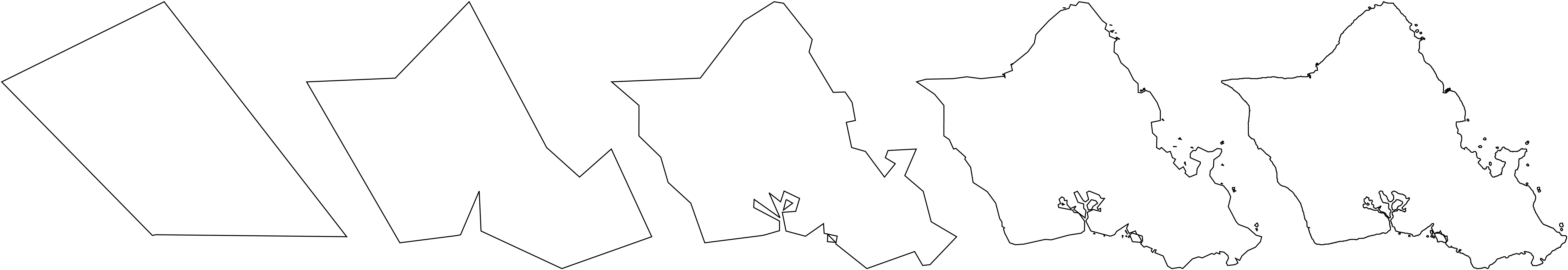
Use the land and water options to specify a fill color for land and water bodies. The colors can be given by name or hex codes:
using GMT
coast(region=:global, proj=:Mollweide, land="#666666", water=:skyblue, show=true)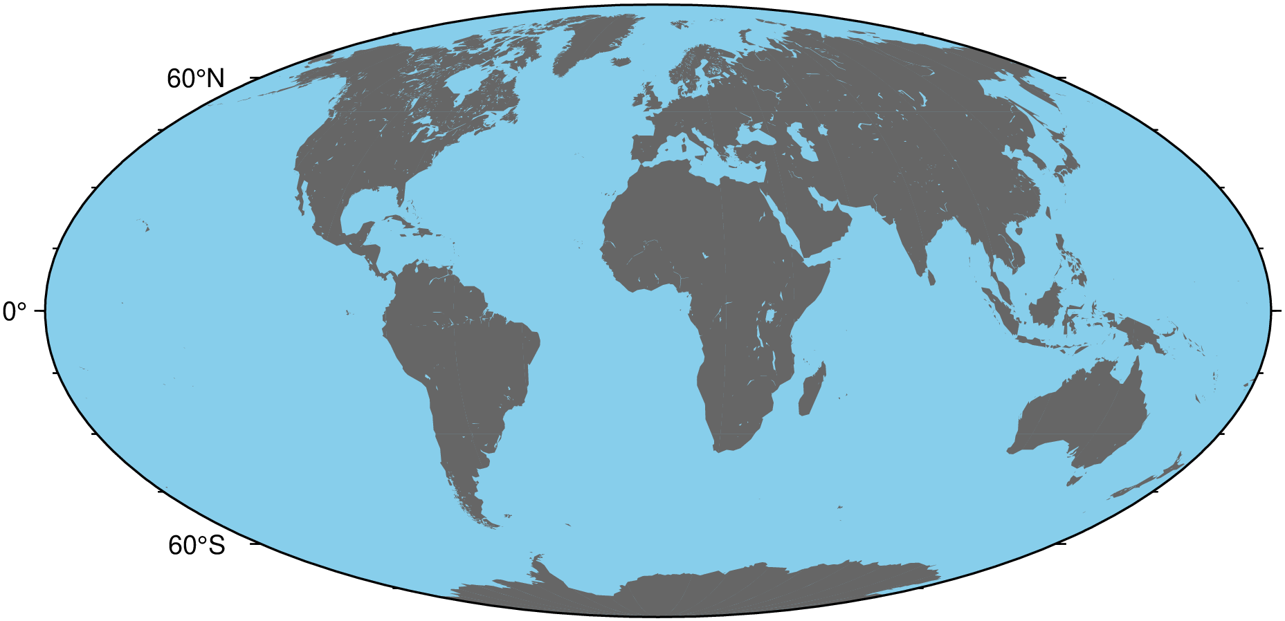
The borders option of coast specifies levels of political boundaries to plot and the pen used to draw them. Choose from the list of boundaries below:
For example, to draw national boundaries with a line thickness of 1p and black line color use borders=(1,("1p",:black)), or borders=(type=1, pen=(0.5, :black)). We can draw multiple boundaries by passing in a tuple of NamedTuples to borders (for repeating the option we must use the NamedTuple form). The following example uses a Sinusoidal projection map of the Americas with automatic annotations and ticks.
using GMT
coast(region=[-150, -30, -60, 60], land=:gray, projection=(name=:Sinusoidal, center=-90),
      borders=((type=1, pen=(0.5, :black)), (type=2, pen=(0.5, :red)), (type=3, pen=(0.5, :blue))),
      show=true)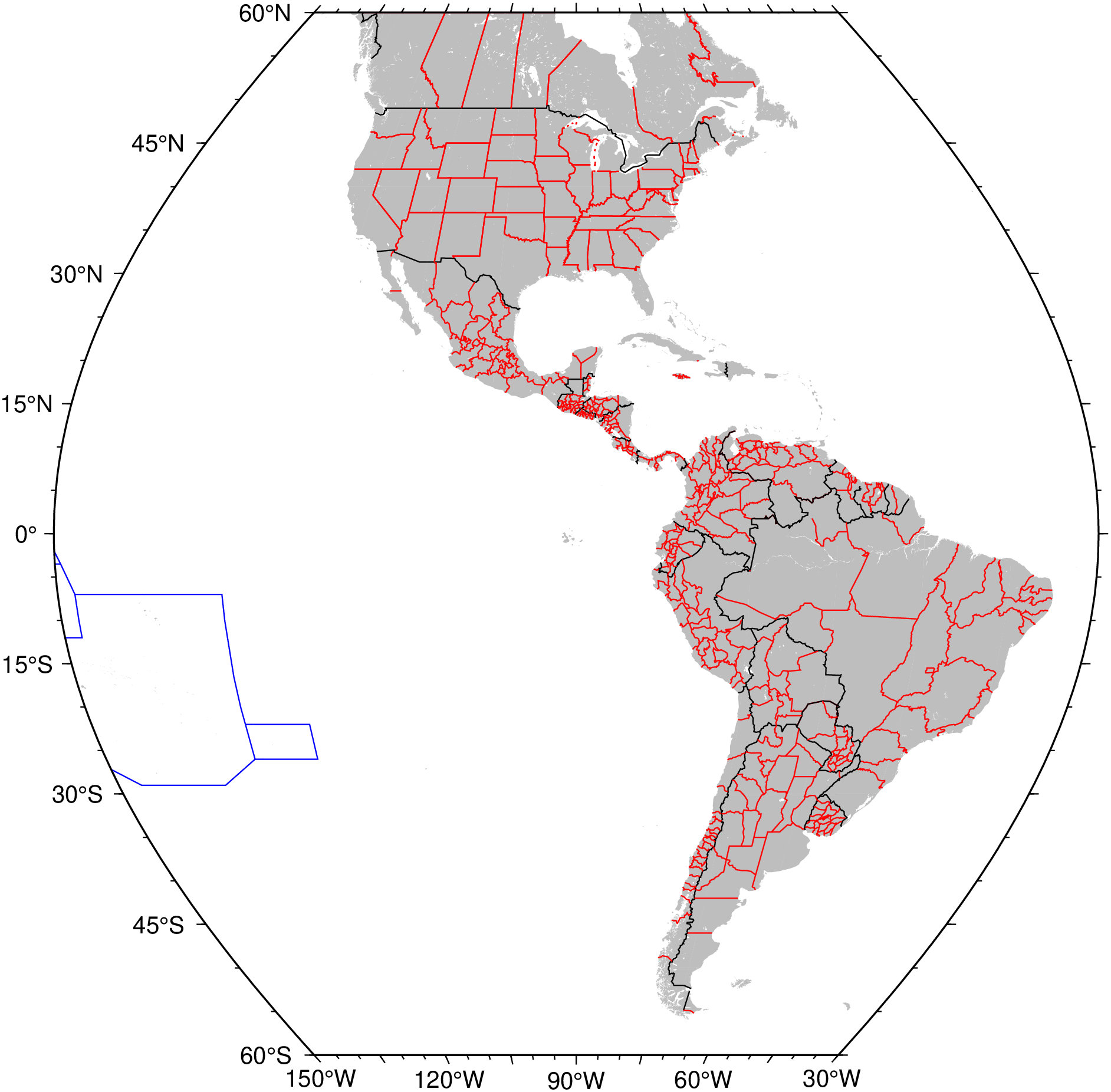
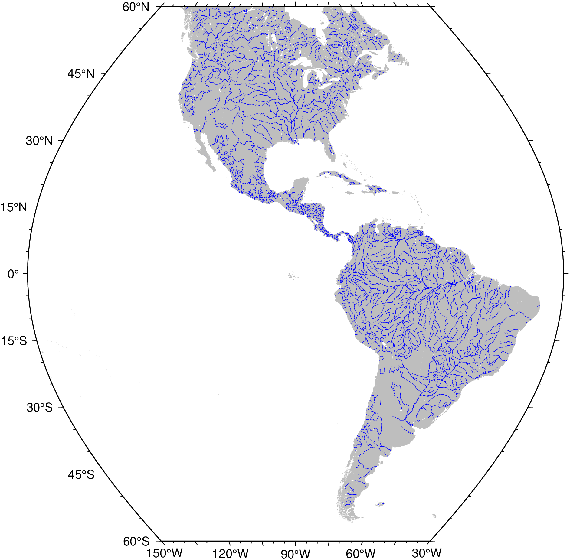
The situation with plotting rivers is a bit less good and we hope to improve it when modern data is incorporated in the databse. But we can still do pretty maps of the permanent major rivers. A rivers version of the figure above is obtained with (the code :r means All permanent rivers):
using GMT
coast(region=[-150, -30, -60, 60], land=:gray, projection=(name=:Sinusoidal, center=-90),
      rivers=(:r,:blue), show=true)