These examples show a GMT.jl version of a PyGMT post in the GMT forum and that can be found at the original author’s, JiahongLuo, Github site
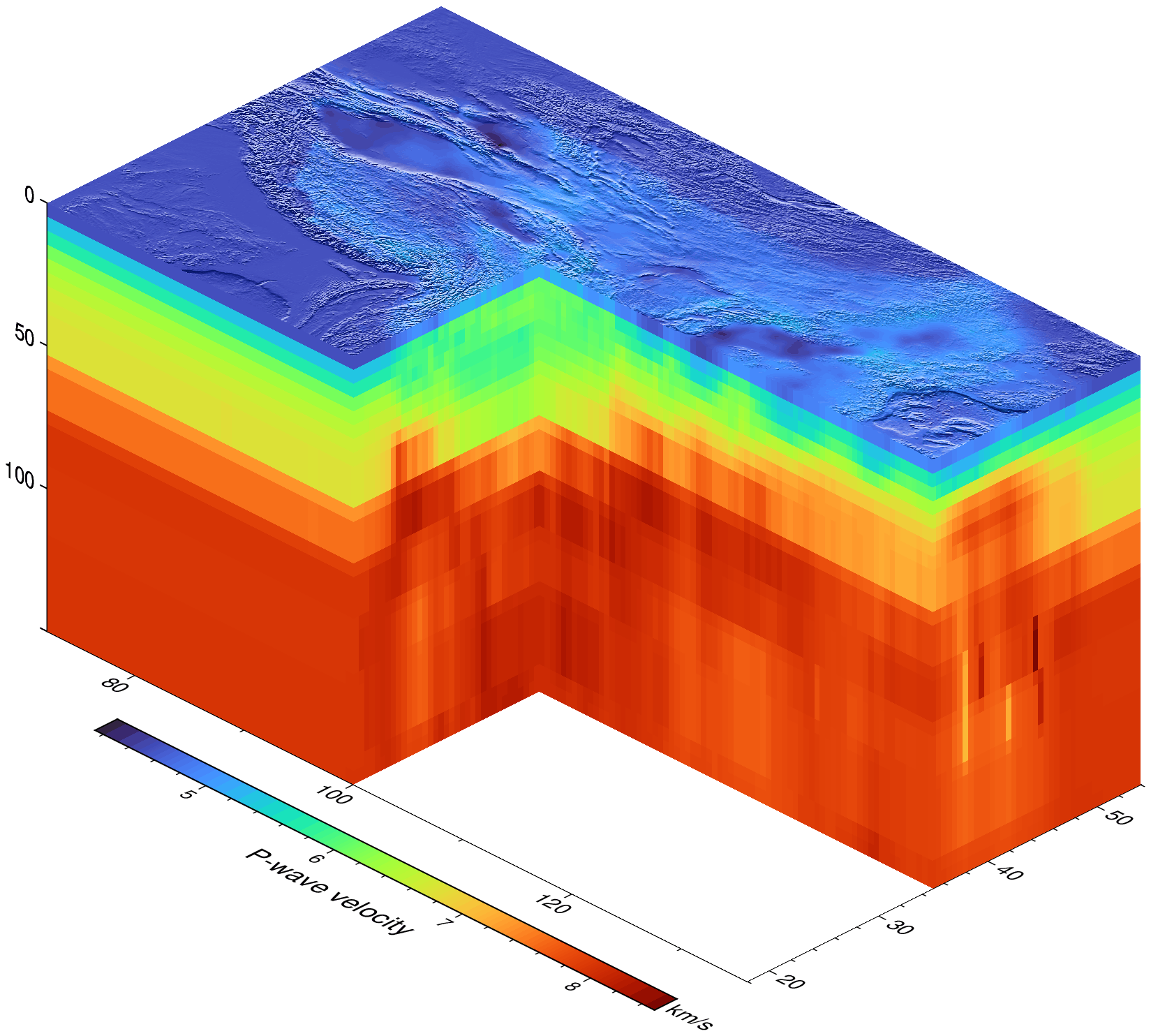
The function let us easily plot images on the sides of a cube. That function can also be used to create those side figures directly from a 3D cube grid.
usingGMT# Download data from:model =gmtread("https://github.com/ShouchengHan/USTClitho2.0/blob/main/USTClitho2.0.wrst.sea_level.txt");# Create two data cubes (grids) with the Vp and Vs velocitiesCvp =xyzw2cube(model);Cvs =xyzw2cube(model, zcol=5);# Add names to the cube layers to be used as titles in next figureCvp.names = ["Depth = $(Int(i)) km" for i in Cvp.v];Cvs.names = ["Depth = $(Int(i)) km" for i in Cvs.v];
gmtread [WARNING]: Long input record (4647 bytes) was truncated to first 4094 bytes!

gmtread [WARNING]: Long input record (4498 bytes) was truncated to first 4094 bytes!

┌ Warning:  file "https://github.com/ShouchengHan/USTClitho2.0/blob/main/USTClitho2.0.wrst.sea_level.txt" is empty or has no data after the header.

└ @ GMT C:\Users\j\.julia\dev\GMT\src\gmtreadwrite.jl:242
The dataset must contain at least 4 columns (x,y,z,w)
Stacktrace:
[1] error(s::String) @Base.\error.jl:35
[2] xyzw2cube(D::GMTdataset{Float64, 2}; zcol::Int64, datatype::DataType, tit::String, names::Vector{String}, varnames::Vector{String}) @GMTC:\Users\j\.julia\dev\GMT\src\utils_types.jl:1818
[3] xyzw2cube(D::GMTdataset{Float64, 2}) @GMTC:\Users\j\.julia\dev\GMT\src\utils_types.jl:1815
[4] top-level scope
@In[2]:4
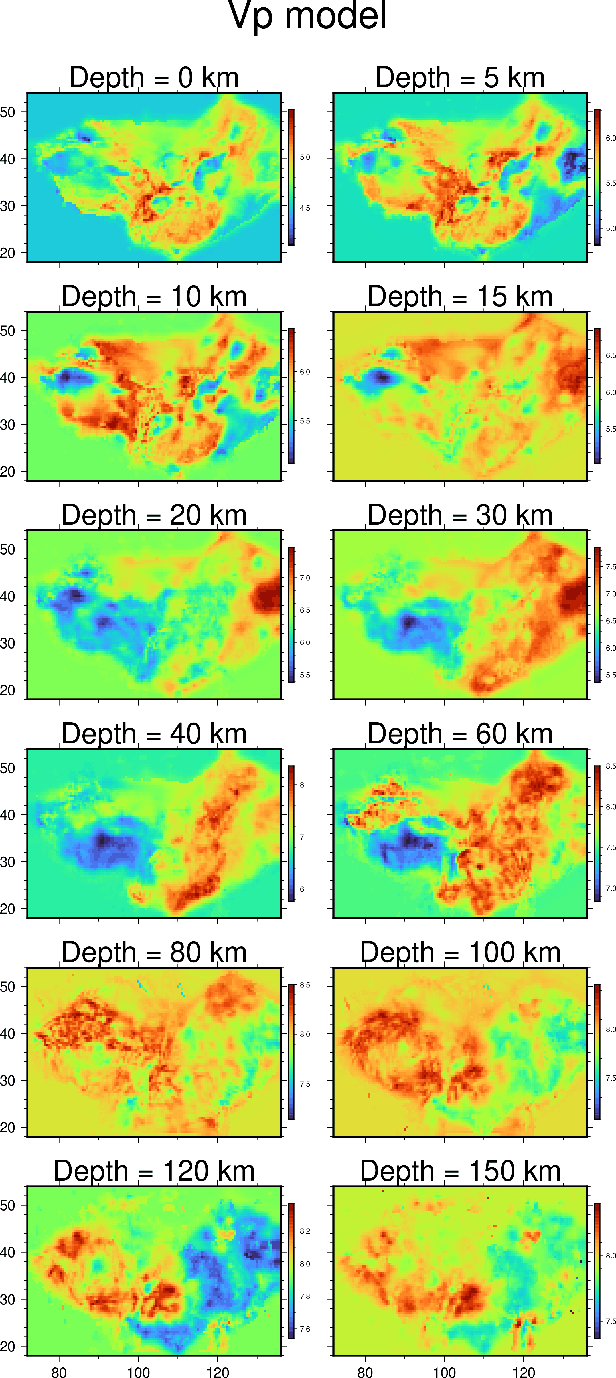
Show all 12 layers of the P-waves velocity in a figure. We use a diffent colormap for each layer to avoid that layers become too monochromatic.
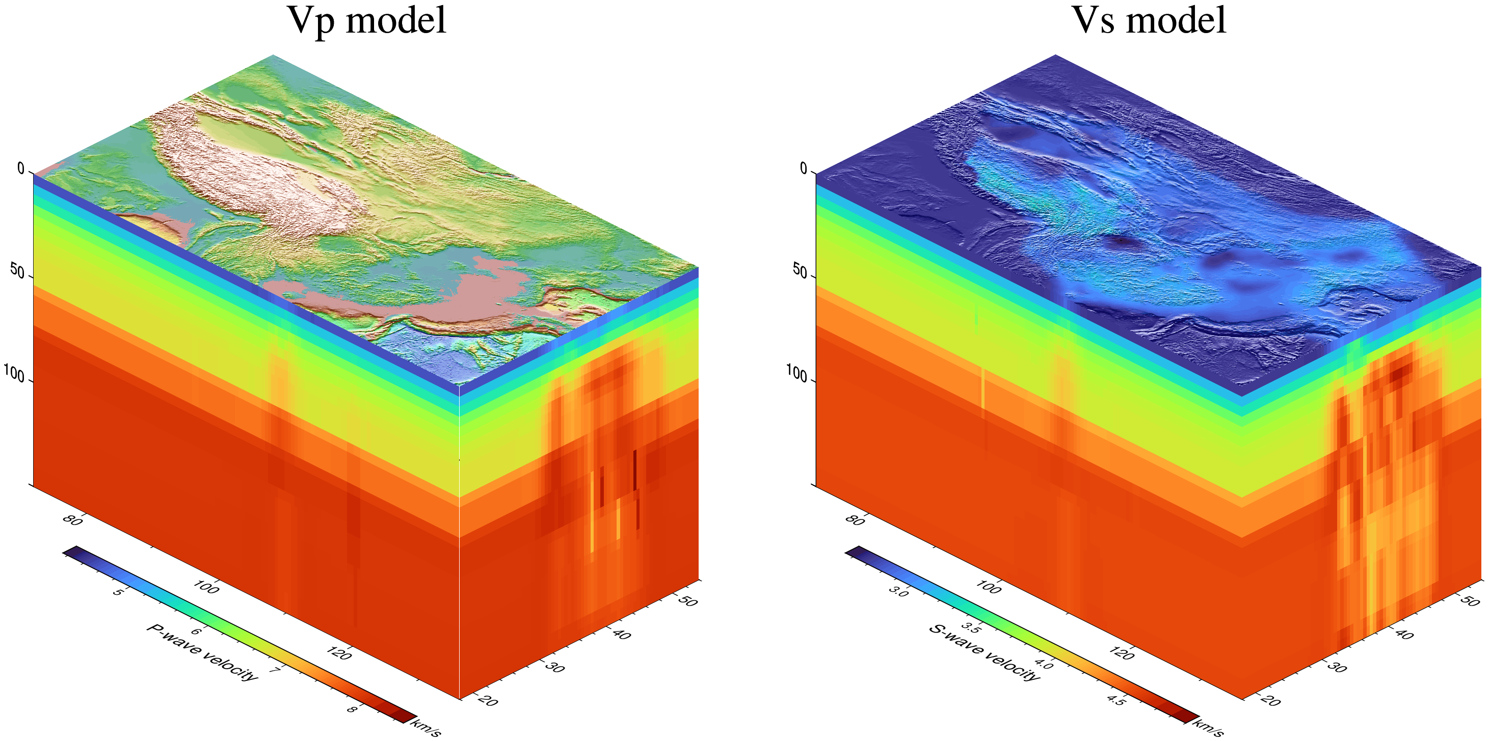
Show the P and S velocities with a slight variation of the top layer. For the P-velocity we plot the topography on top and for the S-velocity we show the superficial S velocity but apply a shading effect calculated from the topography grid.