A or annot : – annot=annot_int | annot=(int=annot_int, disable=true, single=true, labels=labelinfo)
annot_int is annotation interval in data units; it is ignored if contour levels are given in a file. [Default is no annotations]. Use annot=(disable=true,) to disable all annotations implied by cont. Alternatively do annot=(single=true, int=val) to plot val as a single contour. The optional labelinfo controls the specifics of the label formatting and consists of a named tuple with the following control arguments [Label formatting]
B or axes or frame
Set map boundary frame and axes attributes. Default is to draw and annotate left, bottom and vertical axes and just draw left and top axes. More at frame
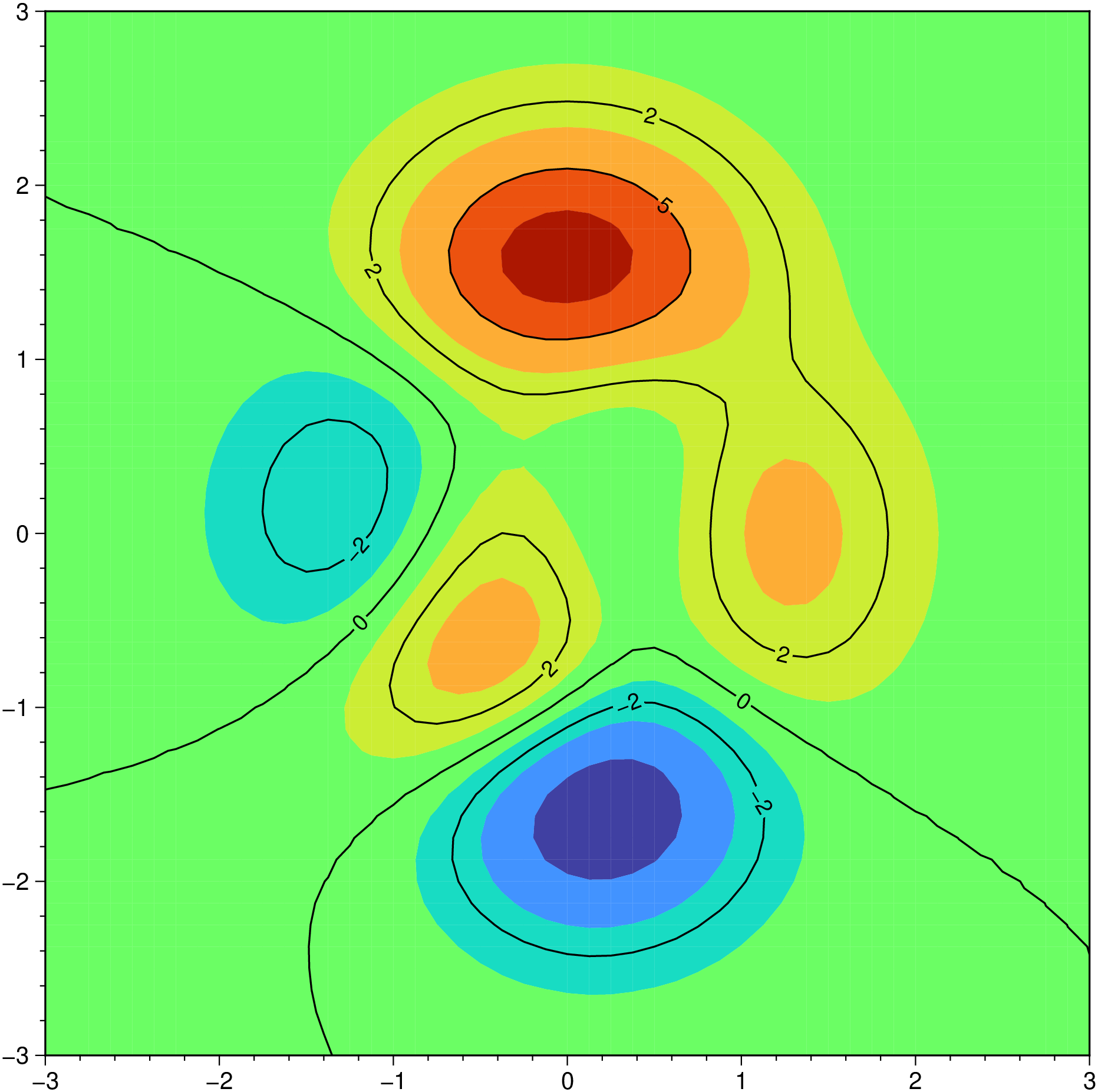
C or cont or contour or contours or levels : – cont=cont_int
The contours to be drawn may be specified in one of two possible ways:
If cont_int is a GMTcpt object (or a string and has the suffix “.cpt” and can be opened as a file). The color boundaries are then used as contour levels. If the CPT has annotation flags in the last column then those contours will be annotated. By default all contours are labeled; use annot=(disable=true,)) (or annot=:none) to disable all annotations.
If cont_int is a constant or an array it means plot those contour intervals. This works also to draw single contours. E.g. contour=[0] will draw only the zero contour. The annot option offers the same possibility so they may be used together to plot a single annotated contour and another single non-annotated contour, as in anot=[10], cont=[5] that plots an annotated 10 contour and an non-annotated 5 contour. If annot is set and cont is not, then the contour interval is set equal to the specified annotation interval.
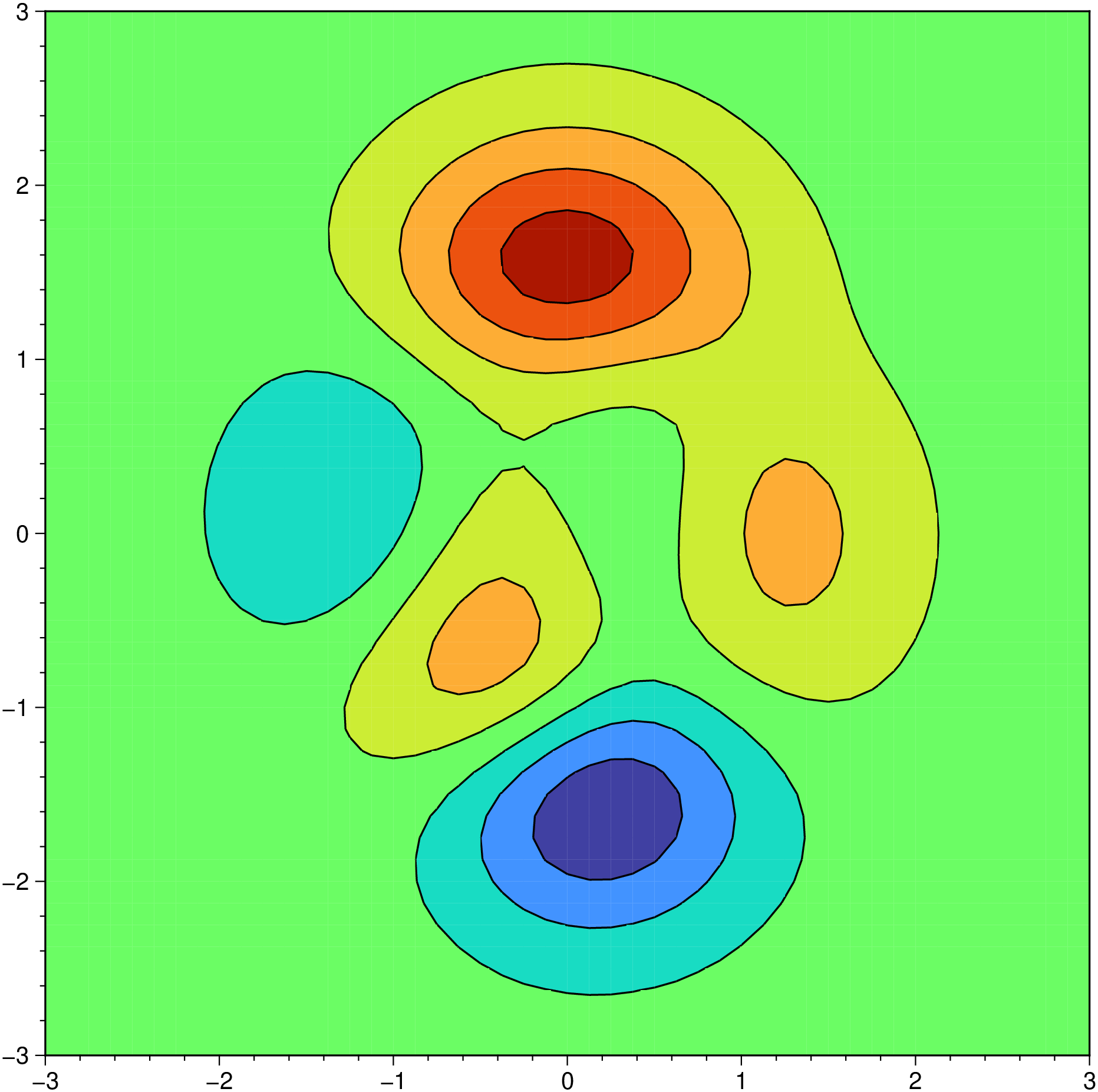
If no contour option and no GMTcpt are passed then for grid a default color map is computed and all of those automatically contours are drwan. Also, no GMTcpt and contour=[array] computes a cmap with only the contour values specified in array. When passing a Mx3 array or a GMTdataset the default behavior is basically the same.
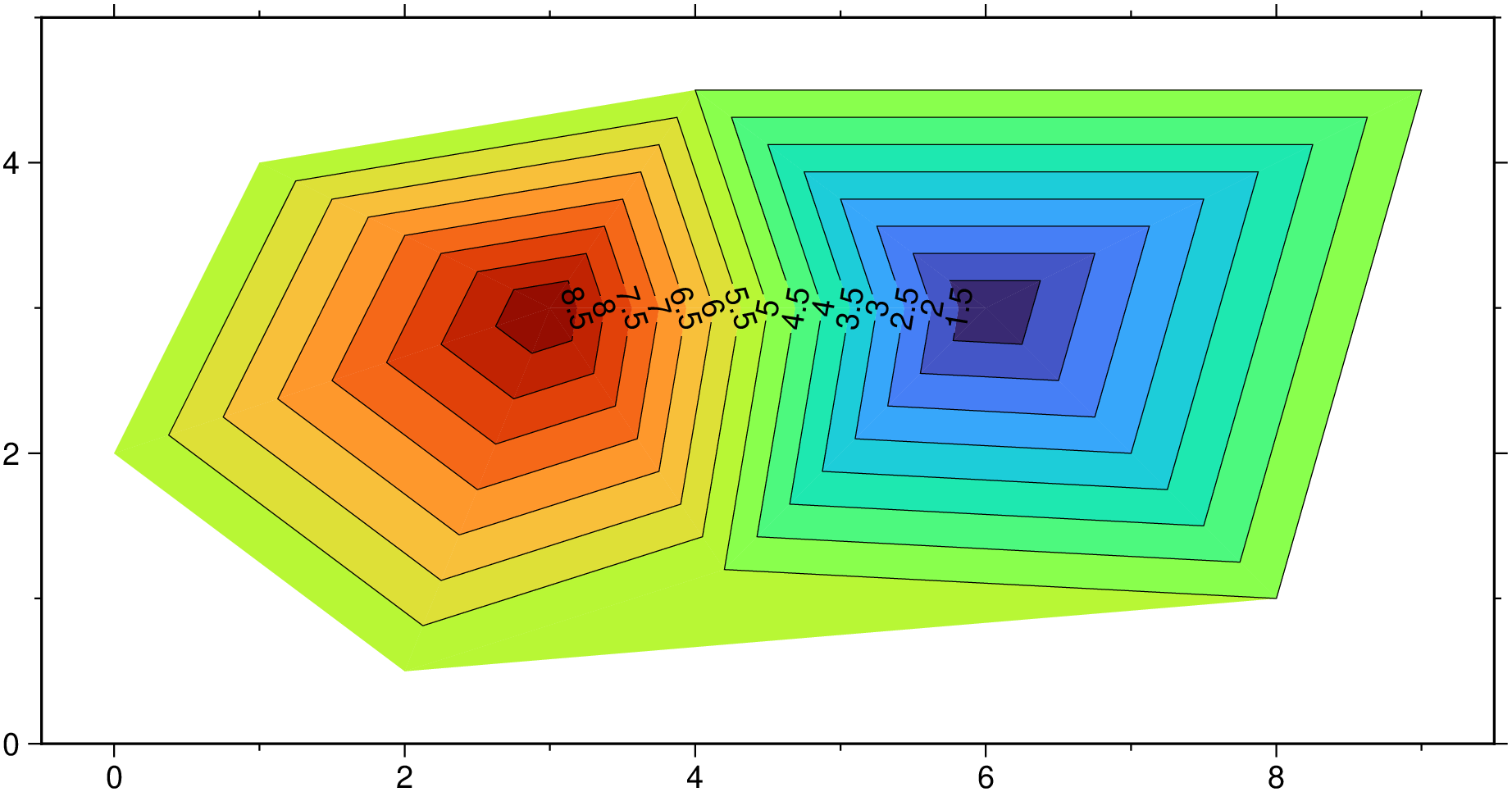
E or index : – index=tri_network
Give a Mx3 array or name of file with network information. Each record must contain triplets of node numbers for a triangle [Default computes these using Delaunay triangulation (see triangulate)].
G or labels : – labels=()
The required argument controls the placement of labels along the quoted lines. Choose among five controlling algorithms as explained in [Label formatting]
J or proj or projection : – proj=
Select map projection. More at proj
Q or cut : – cut=np | cut=length&unit[+z]
Do not draw contours with less than np number of points [Draw all contours]. Alternatively, give instead a minimum contour length in distance units, including c (Cartesian distances using user coordinates) or C for plot length units in current plot units after projecting the coordinates. Optionally, append +z to exclude the zero contour.
R or region or limits : – limits=(xmin, xmax, ymin, ymax) | limits=(BB=(xmin, xmax, ymin, ymax),) | limits=(LLUR=(xmin, xmax, ymin, ymax),units=“unit”) | …more
Specify the region of interest. More at limits. For perspective view view, optionally add zmin,zmax. This option may be used to indicate the range used for the 3-D axes. You may ask for a larger w/e/s/n region to have more room between the image and the axes.
S or smooth : – smooth=smoothfactor
Resample the contour lines at roughly every (gridbox_size/smoothfactor) interval. This option should be used only when input data is a table.
S or skip : – skip=true|“t”
Skip all input xyz points that fall outside the region [Default uses all the data in the triangulation]. Alternatively, use skip=“t” to skip triangles whose three vertices are all outside the region. This option should be used only when input data is a grid.
T or ticks : – ticks=(local_high=true, local_low=true, gap=gap, closed=true, labels=labels)
Will draw tick marks pointing in the downward direction every gap along the innermost closed contours only; set closed=true to tick all closed contours. Use gap=(gap,length) and optionally tick mark length (append units as c, i, or p) or use defaults [“15p/3p”]. User may choose to tick only local highs or local lows by specifying local_high=true, local_low=true, respectively. Set labels to annotate the centers of closed innermost contours (i.e., the local lows and highs). If no labels (i.e, set labels=““) is set, we use - and + as the labels. Appending exactly two characters, e.g., labels=:LH, will plot the two characters (here, L and H) as labels. For more elaborate labels, separate the low and hight label strings with a comma (e.g., labels=“lo,hi”). If a file is given by cont, and ticks is set, then only contours marked with upper case C or A will have tick marks [and annotations].
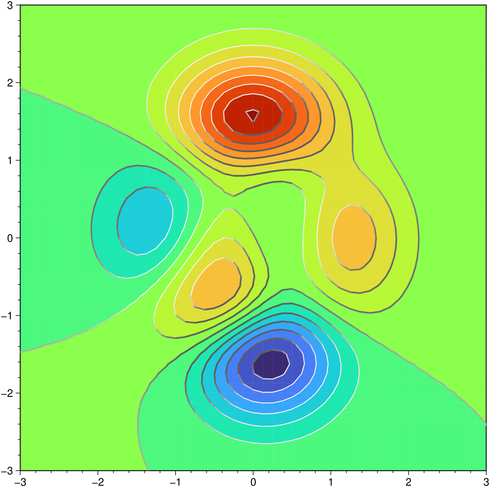
tanaka : – tanaka=true | tanaka=azimuth
Draw Tanaka-style contours with varying line thickness and intensity to simulate illumination from a given direction. The azimuth (in degrees) gives the illumination direction (default is 315 degrees, i.e., NW). Tanaka contours are a bit slow to compute so avoid using this option with large grids.
U or time_stamp : – time_stamp=true | time_stamp=(just=“code”, pos=(dx,dy), label=“label”, com=true)
Draw GMT time stamp logo on plot. More at timestamp
V or verbose : – verbose=true | verbose=level
Select verbosity level. More at verbose
W or pen : – pen=(annot=true, contour=true, pen=pen, colored=true, cline=true, ctext=true)
annot=true if present, means to annotate contours or contour=true for regular contours [Default]. The pen sets the attributes for the particular line. Default pen for annotated contours: pen=(0.75,:black). Regular contours use pen=(0.25,:black). Normally, all contours are drawn with a fixed color determined by the pen setting. This option may be repeated, for example to separate contour and annotated contours settings. For that the syntax changes to use a Tuple of NamedTuples, e.g. pen=((annot=true, contour=true, pen=pen), (annot=true, contour=true, pen=pen)). If the modifier pen=(cline=true,) is used then the color of the contour lines are taken from the CPT (see cont). If instead pen=(ctext=true,) is appended then the color from the cpt file is applied to the contour annotations. Select pen=(colored=true,) for both effects.
X or xshift or x_offset : xshift=true | xshift=x-shift | xshift=(shift=x-shift, mov=“a|c|f|r”)
Shift plot origin. More at xshift
Y or yshift or y_offset : yshift=true | yshift=y-shift | yshift=(shift=y-shift, mov=“a|c|f|r”)
Shift plot origin. More at yshift
p or view or perspective : – view=(azim, elev)
Default is viewpoint from an azimuth of 200 and elevation of 30 degrees.
Specify the viewpoint in terms of azimuth and elevation. The azimuth is the horizontal rotation about the z-axis as measured in degrees from the positive y-axis. That is, from North. This option is not yet fully expanded. Current alternatives are:
- view=??
A full GMT compact string with the full set of options.
- view=(azim,elev)
A two elements tuple with azimuth and elevation
- view=true
To propagate the viewpoint used in a previous module (makes sense only in bar3!) More at perspective
t or transparency or alpha: – alpha=50
Set PDF transparency level for an overlay, in (0-100] percent range. [Default is 0, i.e., opaque]. Works only for the PDF and PNG formats.
figname or savefig or name : – figname=name.png
Save the figure with the figname=name.ext where ext chooses the figure image format.