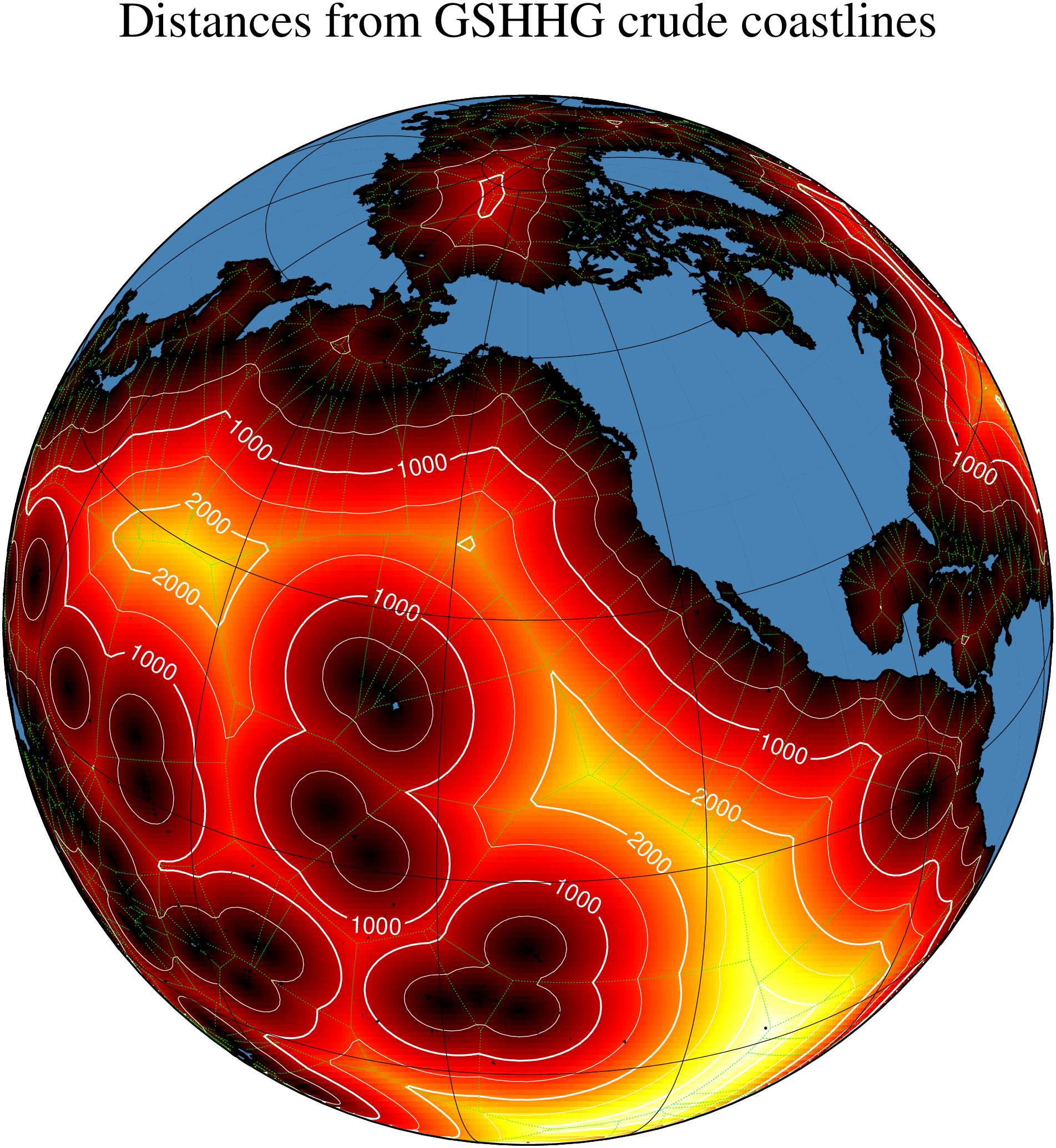
(35) Spherical triangulation and distance calculations

The script produces the plot in Figure. Here we demonstrate how sphtriangulate and sphdistance are used to compute the Delauney and Voronoi information on a sphere, using a decimated GSHHG crude coastline. We show a color image of the distances, highlighted with 500-km contours, and overlay the Voronoi polygons in green. Finally, the continents are placed on top.

using GMT

pol, nodes = sphtriangulate("@gshhs_c.txt", voronoi=:v, skip=true, nodes=true)

# Compute distances in km
Gtt = sphdistance(pol, region=:global360, inc=1, voronoi=true, nodes=nodes, dist_unit=:k)
t_cpt = makecpt(cmap=:hot, range=(0,3500))

# Make a basic image plot and overlay contours, Voronoi polygons and coastlines
grdimage(Gtt, proj=(name=:ortho, center=(-140,30)), figsize=16, xshift=2, yshift=5)
grdcontour!(Gtt, cont=500, annot=(int=1000, labels=(font=(10,:Helvetica,:white),)),
            range=500, labels=(Line=[0 90 203 -10; 175 60 170 -30; -50 30 220 -5],),
            pen=((annot=true, pen=(0.75,:white)), (contour=true, pen=(0.25,:white))) )

plot!(pol, pen=(0.25, :green, :dotted))
coast!(shore=1, land=:steelblue, area=(0,1,1),
       frame=(annot=30, grid=30, title="Distances from GSHHG crude coastlines"), show=true)