plot

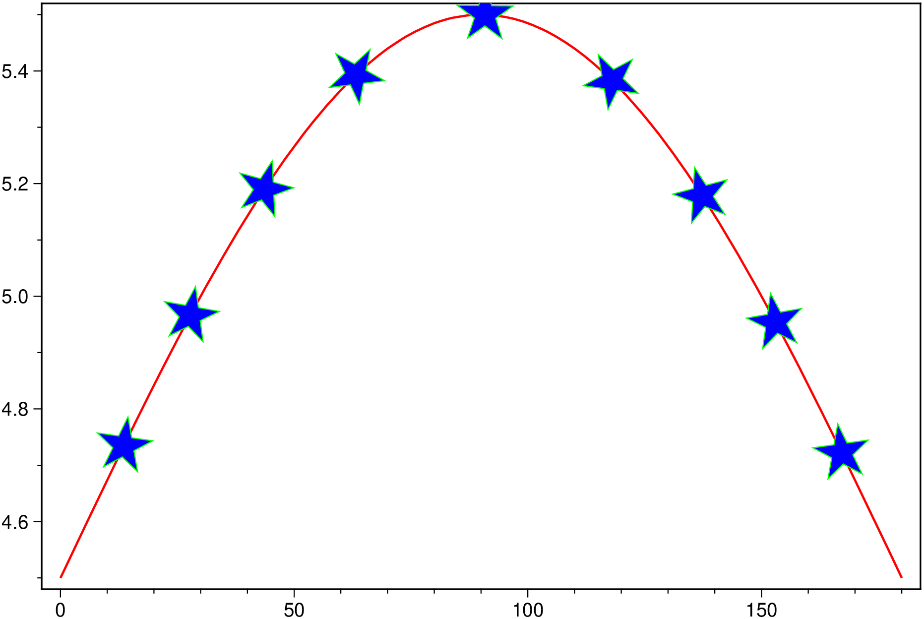
plot(cmd0::String="", arg1=[]; kwargs...)

Reads (x,y) pairs and plot lines, polygons, or symbols with different levels of decoration. The input can either be a file name of a file with at least two columns (x,y),but optionally more, a GMTdatset object with also two or more columns. If a symbol is selected and no symbol size given, then it will interpret the third column of the input data as symbol size. Symbols whose size is <= 0 are skipped. If no symbols are specified then the symbol code (see symbol below) must be present as last column in the input. If symbol is not used, a line connecting the data points will be drawn instead. To explicitly close polygons, use close. Select a fill with fill. If fill is set, pen will control whether the polygon outline is drawn or not. If a symbol is selected, fill and pen determines the fill and outline/no outline, respectively.

Since many options imply further data, to control symbol size and/or color for example, columns beyond 2 for plot or 3 for plot3d cannot be used to plot multiple lines at once (like Matlab does). However, that is stil possible if one uses the form plot(x, y, ...) where x is the coordinates vector or a matrix with only one column or row and y is a matrix with N columns representing the individual lines and M rows, as many as elements in x. This case, off course, looses the possibility of having extra columns with options auxiliary data. Still, another possibility to achieve this when arg1 is a MxN matrix is to use the key/val multicol=true. Automatic legends are obtained by using legend=true.

Selecting both a symbol and a pen plots a line and add the sybols at the vertex.

Parameters

A or steps : – steps=true | steps=:meridian|:parallel|:x|:y|:r|:theta
By default, geographic line segments (as indicated for example by the colinfo option) are drawn as great circle arcs. To draw them as straight lines, use the steps=true. Alternatively, use steps=:meridian to draw the line by first following a meridian, then a parallel. Or append steps=:parallel to start following a parallel, then a meridian. (This can be practical to draw a line along parallels, for example). For Cartesian data, points are simply connected, unless you use steps=:x or steps=:y to draw stair-case curves that whose first move is along x or y, respectively. If your Cartesian data are polar (theta, r), use steps=:t or steps=:r to construct stair-case paths whose first move is along theta or r, respectively.
B or axes or frame
Set map boundary frame and axes attributes. Default is to draw and annotate left, bottom and vertical axes and just draw left and top axes. More at frame
bg or background : – bg=imagename | bg=funname|img|grd | bg=(…, colormap)
Fills the plotting canvas with a backround image. That image may come from a file (e.g. bg=“cute.png”) or from a predefined function name. Possible names are: akley, eggs, circle, parabola, rosenbrok, sombrero, x, y, xy, x+y (see also [Plot surfaces]). In the forms bg=img and bg=grd, the img and grd stand for a GMTimage and a GMTgrid object respectively. Image types can have associated a color map (if they do not, see the [image_cpt!] on how to assign one) but a grid type do not so we need to provide that information in case the turbo default is not intended. To assign a colormap the bg argument must be a two elements tuple, where first element is any of funname|img|grd and the second a colormap name (a CPT) or a GMTcpt object (see also makecpt). To revert the sense of the color progression prefix the colormap name or of the predefined function with a ‘-’. Example: plot(rand(8,2), bg=(:sombrero, "-magma")). Note that the images, either generated or read from file, will normally be deformed to fill the entire area selected with the region option. If that is not wished or if the image coordinates are intended to be used, then this is not the right option but instead you should grdimage followed plot call(s). Another point to notice is that the [frame] option also has a fill or bg|background option that also fills the canvas but it does it using a constant color by replicating a pattern (that can be an image too) and this has a quite different result. The example [Subplots] shows applications of this option.
C or color or cmap : – color=cpt
Give a CPT or specify color=“color1,color2 [,color3 ,…]” or color=((r1,g1,b1),(r2,g2,b2),…) to build a linear continuous CPT from those colors automatically, where z starts at 0 and is incremented by one for each color. In this case color_n can be a [r g b] triplet, a color name, or an HTML hexadecimal color (e.g. #aabbcc ). If symbol is set, let symbol fill color be determined by the z-value in the third column. Additional fields are shifted over by one column (optional size would be 4th rather than 3rd field, etc.). If symbol is not set, then it expects the user to supply a multisegment file where each segment header contains a Zval string. The val will control the color of the line or polygon (if close is set) via the CPT.
D or shift or offset : – offset=(dx,dy) | offset=dx
Offset the plot symbol or line locations by the given amounts dx,dy [Default is no offset]. If dy is not given it is set equal to dx.
E or error or errorbars : – error=(x|y|X|Y=true, notch=true, cap=width, pen=pen, colored=true, cline=true, csymbol=true)
Draw symmetrical error bars. Use error=(x=true) and/or error=(y=true) to indicate which bars you want to draw (Default is both x and y). The x and/or y errors must be stored in the columns after the (x,y) pair [or (x,y,z) triplet]. If asym=true is appended then we will draw asymmetrical error bars; these requires two rather than one extra data column, with the low and high value. If upper case error=(X=true) and/or Y are used we will instead draw “box-and-whisker” (or “stem-and-leaf”) symbols. The x (or y) coordinate is then taken as the median value, and four more columns are expected to contain the minimum (0% quantile), the 25% quantile, the 75% quantile, and the maximum (100% quantile) values. The 25-75% box may be filled by using fill. If notch=true is appended the we draw a notched “box-and-whisker” symbol where the notch width reflects the uncertainty in the median. This symbol requires a 5th extra data column to contain the number of points in the distribution. The cap=width modifier sets the cap width that indicates the length of the end-cap on the error bars [7p]. Pen attributes for error bars may also be set via pen=pen. [Defaults: width = default, color = black, style = solid]. When color is used we can control how the look-up color is applied to our symbol. Add cline=true to use it to fill the symbol, while csymbol=true will just set the error pen color and turn off symbol fill. Giving colored=true will set both color items.
F or conn or connection : – conn=(continuous=true, net|network=true, refpoint=true, ignore_hdr=true, single_group=true, segments=true, anchor=(x,y))
Alter the way points are connected (by specifying a scheme) and data are grouped (by specifying a method). Use one of three line connection schemes:
- continuous=true : Draw continuous line segments for each group [Default].
- refpoint=true : Draw line segments from a reference point reset for each group.
- network=true : Draw networks of line segments between all points in each group. Optionally, use one of four segmentation methods to define the group:
- ignore_hdr=true : Ignore all segment headers, i.e., let all points belong to a single group, and set group reference point to the very first point of the first file.
- single_group=true : Consider all data in each file to be a single separate group and reset the group reference point to the first point of each group.
- segments=true : Segment headers are honored so each segment is a group; the group reference point is reset to the first point of each incoming segment [Default].
- segments_reset=true : Same as segments=true, but the group reference point is reset after each record to the previous point (this method is only available with the refpoint=true scheme). Instead of the codes ignore_hdr, single_group, segments, segments_reset you may append the coordinates of a anchor=(x,y) which will serve as a fixed external reference point for all groups.
J or proj or projection : – proj=
Select map projection. More at proj
Jz or JZ or zscale or zsize (for plot3d only) : – zscale=scale | zsize=size
Set z-axis scaling or or z-axis size. zsize=size sets the size to the fixed value size (for example zsize=10 or zsize=4i). zscale=scale sets the vertical scale to UNIT/z-unit.
R or region or limits : – limits=(xmin, xmax, ymin, ymax) | limits=(BB=(xmin, xmax, ymin, ymax),) | limits=(LLUR=(xmin, xmax, ymin, ymax),units=“unit”) | …more
Specify the region of interest. More at limits. For perspective view view, optionally add zmin,zmax. This option may be used to indicate the range used for the 3-D axes. You may ask for a larger w/e/s/n region to have more room between the image and the axes.
G or markerfacecolor or MarkerFaceColor or markercolor or mc or fill
Select color or pattern for filling of symbols [Default is no fill]. Note that plot will search for fill and pen settings in all the segment headers (when passing a GMTdaset or file of a multi-segment dataset) and let any values thus found over-ride the command line settings (but those must be provided in the terse GMT syntax). See Setting color for extend color selection (including color map generation).
hexbin : – hexbin=true
Make a 2D hexagonal binning plot of points xy that have been processed by binstats(xy, tiling=:hex, stats=...). Note thatb for this we rely in keeping a correct trac of the figure size and plot limis, which is not obvious because those are often given as strings and we must parse them back to numeric. In case it fails, it’s users responsability to provide a correct size to the marker=hexagon, markersize=??? options.
I or shade : – shade=intens
Use the supplied intens value (nominally in the -1 to +1 range) to modulate the fill color by simulating illumination [none]. If no intensity is provided (e.g. shade=““) we will instead read intens from the first data column after the symbol parameters (if given).
L or close or polygon : – close=(sym=true, asym=true, envelope=true, left=true, right=true, x0=x0, top=true, bot=true, y0=y0, pen=pen)
Force closed polygons. Alternatively, add modifiers to build a polygon from a line segment.
- sym=true to build symmetrical envelope around y(x) using deviations dy(x) given in extra column 3.
- asym=true to build asymmetrical envelope around y(x) using deviations dy1(x) and dy2(x) from extra columns 3-4.
- envelope=true to build asymmetrical envelope around y(x) using bounds yl(x) and yh(x) from extra columns 3-4.
- left=true or right=true or x0=x0 to connect first and last point to anchor points at either xmin, xmax, or x0, or
- bot=true or top=true or y0=y0 to connect first and last point to anchor points at either ymin, ymax, or y0. Polygon may be painted (fill) and optionally outlined by adding pen=pen. See also the ribbon option further down.
N or noclip or no_clip : noclip=true | noclip=:r | noclip=:c
Do NOT clip symbols that fall outside map border [Default plots points whose coordinates are strictly inside the map border only]. This option does not apply to lines and polygons which are always clipped to the map region. For periodic (360-longitude) maps we must plot all symbols twice in case they are clipped by the repeating boundary. The noclip will turn off clipping and not plot repeating symbols. Use noclip=:r to turn off clipping but retain the plotting of such repeating symbols, or use noclip=:c to retain clipping but turn off plotting of repeating symbols.
S or symbol or marker : – symbol=(symb=name, size=val, unit=unity) or marker|Marker|shape=name, markersize|MarkerSize|ms|size=val
Plot symbols (including vectors, pie slices, fronts, decorated or quoted lines). If present, size is symbol size in the unit set in gmt.conf (unless c, i, or p is appended to markersize or synonym or cm, inch, point as unity when using the symbol=(symb=name,size=val,unit=unity) form). If the symbol name is not given it will be read from the last column in the input data (must come from a file name or a GMTdataset); this cannot be used in conjunction with binary input (data from file). Optionally, append c, i,or p to indicate that the size information in the input data is in units of cm, inch, or point, respectively [Default is PROJ_LENGTH_UNIT]. Note: if you provide both size and symbol via the input file you must use PROJ_LENGTH_UNIT to indicate the unit used for the symbol size or append the units to the sizes in the file. If symbol sizes are expected via the third data column then you may convert those values to suitable symbol sizes via the incol mechanism.
You can change symbols by adding the required -S option to any of your multisegment headers (GMTdataset only). Choose between these symbol codes:
- - or x-dash size is the length of a short horizontal (x-dir) line segment.
- + or plus size is diameter of circumscribing circle.
- a or * or star size is diameter of circumscribing circle.
- c or circle size is diameter of circle.
- d or diamond size is diameter of circumscribing circle.
- e or ellipse Direction (in degrees counter-clockwise from horizontal), major_axis, and minor_axis must be found in columns 3, 4, and 5.
- E or Ellipse Same as ellipse, except azimuth (in degrees east of north) should be given instead of direction. The azimuth will be mapped into an angle based on the chosen map projection (ellipse leaves the directions unchanged.) Furthermore, the axes lengths must be given in geographical instead of plot-distance units. An exception occurs for a linear projection in which we assume the ellipse axes are given in the same units as region. For degenerate ellipses (circles) with just the diameter given, use Ellipse-. The diameter is excepted to be given in column 3. Alternatively, append the desired diameter to E- and this fixed diameter is used instead (e.g. symbol=“E-500”). For allowable geographical units, see UNITS.
- front Draw a front. See [Front lines]
- g or octagon size is diameter of circumscribing circle.
- h or hexagon size is diameter of circumscribing circle.
- i or inverted_tri size is diameter of circumscribing circle.
- j or rotated_rec Rotated rectangle. Direction (in degrees counter-clockwise from horizontal), x-dimension, and y-dimension must be found in columns 3, 4, and 5.
- J or Rotated_rec Same as rotated_rec, except azimuth (in degrees east of north) should be given instead of direction. The azimuth will be mapped into an angle based on the chosen map projection (rotated_rec leaves the directions unchanged.) Furthermore, the dimensions must be given in geographical instead of plot-distance units. For a degenerate rectangle (square) with one dimension given, use J-. The dimension is excepted to be given in column 3. Alternatively, append the dimension diameter to J- and this fixed dimension is used instead. An exception occurs for a linear projection in which we assume the dimensions are given in the same units as region. For allowable geographical units, see UNITS.
- m or matang math angle arc, optionally with one or two arrow heads [Default is no arrow heads]. The size is the length of the vector head. Arc width is set by pen, with vector head outlines defaulting to half of arc width. The radius of the arc and its start and stop directions (in degrees counter-clockwise from horizontal) must be given in columns 3-5. See [Vector Attributes] for specifying other attributes.
- M or Matang Same as matang but switches to straight angle symbol if angles subtend 90 degrees exactly.
- n or pentagon size is diameter of circumscribing circle.
- p or point No size needs to be specified (1 pixel is used).
- quoted lines i.e., lines with annotations such as contours. See [Quoted lines]
- r or rectangle No size needs to be specified, but the x- and y-dimensions must be found in columns 3 and 4.
- R or roundrect Rounded rectangle. No size needs to be specified, but the x- and y-dimensions and corner radius must be found in columns 3, 4, and 5.
- s or square size is diameter of circumscribing circle.
- t or ^ or triangle size is diameter of circumscribing circle.
- w or wedge or web or pie size is diameter of circumscribing circle. Data is x,y (center) startdir and stopdir
- W or Wedge or Web or Pie Same as wedge, except azimuths (in degrees east of north) should be given instead of the two directions.
- x or cross size is diameter of circumscribing circle.
- y or y-dash (|). size is the length of a short vertical (y-dir) line segment.
- decorated i.e., lines with symbols along them. See [Decorated lines]
csymbol or cmarker or custom_symbol or custom_marker : – csymbol=(name=symbname, size=val, unit=unity)
Use one the GMT’s custom symbols where symbname is the lowercase name of any of those in the table, plus arrow or ski_alpine (these are from GMT.jl).
W or pen=pen
Set pen attributes for lines or the outline of symbols [Defaults: width = default, color = black, style = solid]. See [Pen attributes]. If the modifier pen=(cline=true) is appended then the color of the line are taken from the CPT (see cmap). If instead modifier pen=(csymbol=true) is appended then the color from the cpt file is applied to symbol fill. Use pen=(colored=true) for both effects. You can also append one or more additional line attribute modifiers: offset=val will start and stop drawing the line the given distance offsets from the end point. Append unit u from c | i | p to indicate plot distance on the map or append map distance units instead (see below); bezier=true will draw the line using a Bezier spline; vspecs will place a vector head at the ends of the lines. You can use vec_start and vec_stop to specify separate vector specs at each end [shared specs]. See the [Vector Attributes] for more information. If level is set, then pen=(zlevels=true) assign pen color via cmap and the z-values obtained. Finally, if pen color = :auto then we will cycle through the pen colors implied by COLOR_SET and change on a per-segmentbasis. The width, style, or transparency settings are unchanged.
decimate : – decimate=true | decimate=decfactor
For very large datasets it may be convenient to decimate data before plotting. The decimate option decimates the input data using a clever algorithm (see MS-thesis). The decfactor (default is 10) is used such that the decimated size is 1÷decfactor of initial size.
groupvar or hue : – groupvar=“text” | groupvar=Int | groupvar=:ColName
Uses the table variable specified by groupvar to group the points in the plot. groupvar can be a column number, or a column name passed in as a Symbol. e.g. groupvar=:Male if a column with that name exists. When arg1 is GMTdatset or cmd0 is the name of a file with one and it has the text field filled, use groupvar="text" or groupvar=*text_col_name* to use that text field as the grouping vector.
legend and label : – legend=“thelabel” | label=thelabel | legend=(label=“thelabel”, pos=position, box=??, fontsise=?, font=?)
Add a legend to the plot. In its simple form just provide legend="thelabel", which plots the legend at the default UpperRight position. To control the legend position and other parameters one must use the tuple form where label="thelabel" is the same as above; pos=position where position is a 2 char code (or its expanded form) like in the text. For a full featured positioning option in legend=(label="thelabel", pos=(...)) see the pos option in legend that allows also to plot the legend outside of the figure space. The box option may take two forms (refer to legend for more details): (1) use box=:none to not plot the legend box or,
1. box=(clearance=?, fill=?, inner=?, pen=?, rounded=?, shade=?). For example, box=(pen=1, fill="gray95", shade=true) to plot a light gray box with a shade. When using the groupvar option we can just set legend=true to create a legend containing an entry for each of the groups. Controling the position of that legend is done by omitting the label keyword in the legend=(...) form. e.g. legend=(pos=:TL,). Use fontsise=?, where ? is the size in points, controls the legend text size and font=? to change the default font. Example: label=(fontsize=8, font="Helvetica,blue")
linefit or regress : – linefit=true
Plot a regression fit over a scatter plot. Input can either be a GMTdataset obtained from the linearfitxy function or a Mx2 matrix. Preferably use the first form that provides more user control. See the linearfitxy documentation for extra options usable in this case.
ribbon or band : – ribbon=dy | ribbon=(dy1,dy2) | *ribbon=mat | ribbon=(vec1,vec2)
Similar to the polygon** option above but where the data to build envelope around y(x) is passed directly via this option instead of extra columns in the input data. In the above dy, dy1, dy2 are scalars, mat is a Mx2 matrix and vec1,vec2 are vectors with the same length as number of rows in input data.
zcolor or markerz or mz : – zcolor=xx | zcolor=true
Take the vector xx (same size as number os points in data) and interpolate the current color scale to paint the symbols based on that colr scale. The form zcolor=true is equivant to zcolor=1:npoints
U or time_stamp : – time_stamp=true | time_stamp=(just=“code”, pos=(dx,dy), label=“label”, com=true)
Draw GMT time stamp logo on plot. More at timestamp
V or verbose : – verbose=true | verbose=level
Select verbosity level. More at verbose
X or xshift or x_offset : xshift=true | xshift=x-shift | xshift=(shift=x-shift, mov=“a|c|f|r”)
Shift plot origin. More at xshift
Y or yshift or y_offset : yshift=true | yshift=y-shift | yshift=(shift=y-shift, mov=“a|c|f|r”)
Shift plot origin. More at yshift
Z or level : level=vec | level=(data=vec, outline=true, nofill=true) | level=“att=???”
Instead of specifying a symbol or polygon fill and outline color via markercolor and pen, give both a value via level and a color lookup table via color. Alternatively, give a vector with one z-value for each polygon in the input data. To apply it to the pen color, use level=(data=vec, outline=true). This results in filled polygons and outline color chosen from the vec and the active cmap. Use level=(data=vec, nofill=true) to only paint outlines but not fill. Instead of a numeric vec, one can pass an attribute name of the attrib holding the numeric data in the GMTdaset. For example, this is legal too: level=(data=“att=FROMAGE”, nofill=true). Here, the contents of the FROMAGE attribute will be used to color lines or polygons. The default is to fill and draw outlines with default color (black). This option is particularly useful to make choropleth maps. Note, options fill and pen may overlap with this option.
figname or savefig or name : – figname=name.png
Save the figure with the figname=name.ext where ext chooses the figure image format.

Units

For map distance unit, append unit d for arc degree, m for arc minute, and s for arc second, or e for meter [Default], f for foot, k for km, M for statute mile, n for nautical mile, and u for US survey foot. By default we compute such distances using a spherical approximation with great circles (spheric_dist=:g). You can use spheric_dist=:f to perform “Flat Earth” calculations (quicker but less accurate) or spheric_dist=:e to perform exact geodesic calculations (slower but more accurate; see PROJ_GEODESIC for method used).

Examples

Decorated curve with blue stars

using GMT

xy = gmt("gmtmath -T0/180/1 T SIND 4.5 ADD");
lines(xy, axes=:af, pen=(1,:red), decorated=(dist=(2.5,0.25), symbol=:star,
      ms=1, pen=(0.5,:green), fill=:blue, dec2=true), show=true)