using GMT
resetGMT() # hide
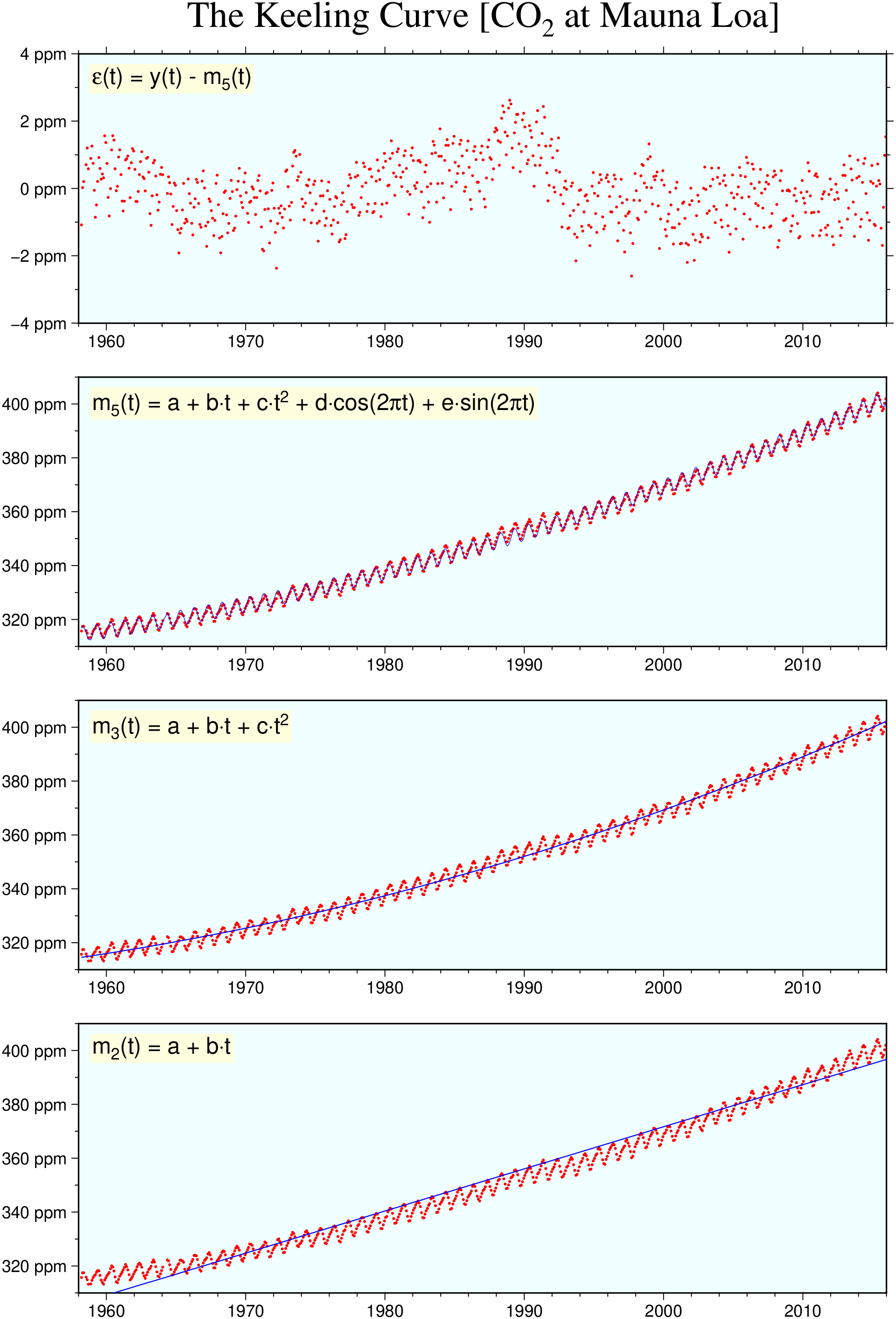
# Basic LS line y = a + bx
model = trend1d("@MaunaLoa_CO2.txt", output=:xm, model=:p1)
plot("@MaunaLoa_CO2.txt", region=(1958,2016,310,410), frame=(axes=:WSen, bg=:azure1),
xaxis=(annot=:auto, ticks=:auto), yaxis=(annot=:auto, ticks=:auto, suffix=" ppm"),
marker=:circle, ms=0.05, fill=:red, figsize=(15,5), xshift=4)
plot!(model, pen=(0.5,:blue))
text!(mat2ds("m@-2@-(t) = a + b@~\\327@~t"), font=12, region_justify=:TL,
offset=(away=true, shift=0.25), fill=:lightyellow)
# Basic LS line y = a + bx + cx^2
model = trend1d("@MaunaLoa_CO2.txt", output=:xm, model=:p2)
plot!("@MaunaLoa_CO2.txt", frame=:same, ms=0.05, fill=:red, yshift=6)
plot!(model, pen=(0.5,:blue))
text!(mat2ds("m@-3@-(t) = a + b@~\\327@~t + c@~\\327@~t@+2@+"), font=12,
region_justify=:TL, offset=(away=true, shift=0.25), fill=:lightyellow)
# Basic LS line y = a + bx + cx^2 + seasonal change
model = trend1d("@MaunaLoa_CO2.txt", output=:xmr, model="p2,f1+o1958+l1")
plot!("@MaunaLoa_CO2.txt", frame=:same, ms=0.05, fill=:red, yshift=6)
plot!(model, pen=(0.25,:blue))
text!(mat2ds("m@-5@-(t) = a + b@~\\327@~t + c@~\\327@~t@+2@+ + d@~\\327@~cos(2@~p@~t) + e@~\\327@~sin(2@~p@~t)"),
font=12, region_justify=:TL, offset=(away=true, shift=0.25), fill=:lightyellow)
# Plot residuals of last model
plot!(model, region=(1958,2016,-4,4), frame=(axes=:WSen, bg=:azure1,
title="The Keeling Curve [CO@-2@- at Mauna Loa]"), xaxis=(annot=:auto, ticks=:auto),
yaxis=(annot=:auto, ticks=:auto, suffix=" ppm"),
ms=0.05, fill=:red, incols="0,2", yshift=6)
text!(mat2ds("@~e@~(t) = y(t) - m@-5@-(t)"), font=12, region_justify=:TL,
offset=(away=true, shift=0.25),fill=:lightyellow, show=true)