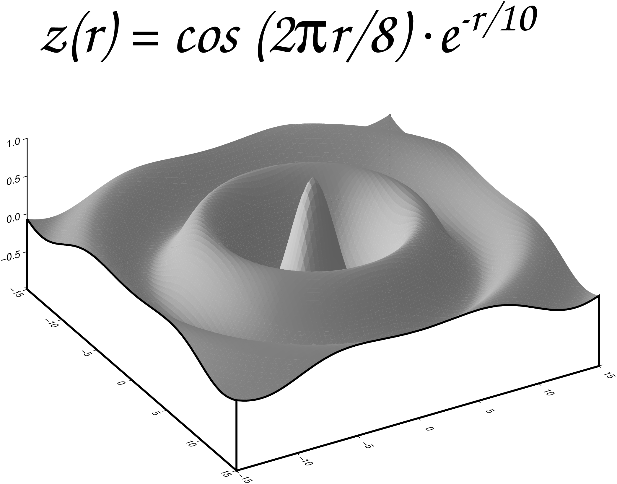
Instead of a mesh plot we may choose to show 3-D surfaces using artificial illumination. For this example we will use grdmath to make a grid file that contains the surface given by the function , where . The illumination is obtained by passing the grid file to [grdview] and requesting that artificial shading be derived from the horizontal gradients in the direction of the artificial light source. The [makecpt] command creates a simple color scheme for a constant gray level of 128. Thus, variations in shade are entirely due to variations in gradients, or illuminations. We choose to illuminate from the SW and view the surface from SE:
The variations in intensity could be made more dramatic by using grdmath to scale the intensity file before running [grdview]. For very rough data sets one may improve the smoothness of the intensities by computing them first with [grdgradient] and then pass them to [grdhisteq]. The shell-script above will result in a plot like the one in Figure.
usingGMTresetGMT() # hideGsombrero =gmt("grdmath -R-15/15/-15/15 -I0.3 X Y HYPOT DUP 2 MUL PI MUL 8 DIV COS EXCH NEG 10 DIV EXP MUL =");C =makecpt(color=128, range=(-5,5), no_bg=true);grdview(Gsombrero, limits=(-15,15,-15,15,-1,1), frame=(axes="SEwnZ", annot=5), zaxis=(annot=0.5,), plane=(-1, :white), surftype=:surface, shade=(azim=225, norm="t0.75"), figsize=12, zsize=5, view=(120,30))tit =mat2ds([7.512], "z(r) = cos (2@~p@~r/8) @~\\327@~e@+-r/10@+");text!(tit, limits=(0,21,0,28), proj=:linear, view=:none, font=(50,"ZapfChancery-MediumItalic"), justify=:CB, scale=1, show=true)