FFT example I

Example on how to decompose and filter a synthetic time series with Fourier analysis.

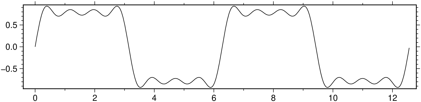
func(x) = sin(x) + 1/3*sin(3x) + 1/5*sin(5x) + 1/7*sin(7x);
x = 0:0.01:4pi;

Evaluate func at x and plot its value.

y = func.(x);
viz(x,y, figsize=(14,3))

Fs = 50000;     # Sampling frequency
T = 1/Fs;       # Sampling period
L = 10000;      # Length of signal
t = (0:L-1)*T;  # Time vector

A1 = 325;		# Amplitude of first sinusoid
f1 = 50;		   # Frequency of first sinusoid
A2=200;			# Amplitude of second sinusoid
f2=400;			# Frequency of second sinusoid
A3=150;			# Amplitude of third sinusoid
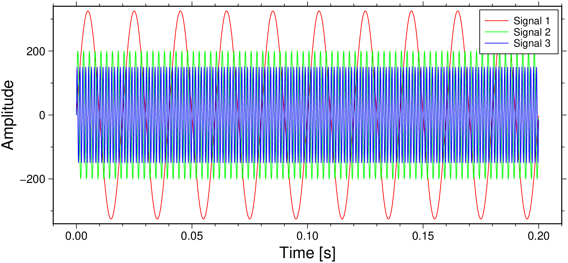
f3=800;			# Frequency of third sinusoid

Generate three sine waves with different frequencies and amplitudes.

using GMT, FFTW

sig1 = A1*sin.(2*pi*f1*t);
sig2 = A2*sin.(2*pi*f2*t);
sig3 = A3*sin.(2*pi*f3*t);
plot(t, sig1, xlabel="Time [s]", ylabel="Amplitude", label="Signal 1", lc=:red, figsize=(14,6))
plot!(t, sig2, label="Signal 2", lc=:green)
plot!(t, sig3, label="Signal 3", lc=:blue, show=true)

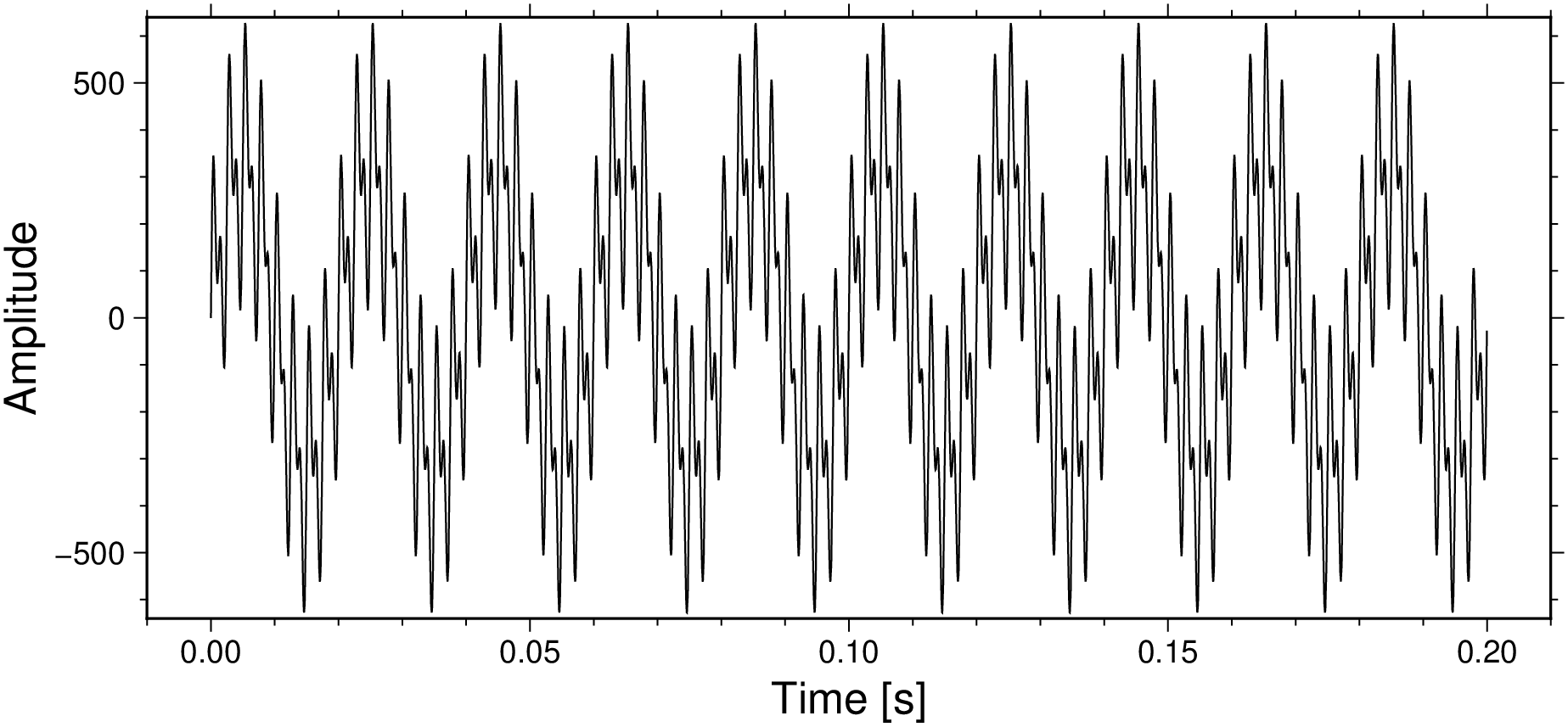
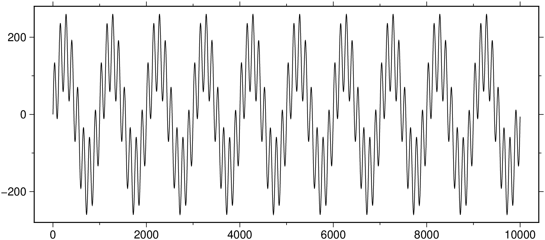
Add the three signals together and plot the result.

final= sig1 .+ sig2 .+ sig3;	# Add the three signals together
plot(t, final, xlabel="Time [s]", ylabel="Amplitude", figsize=(14,6), show=1)

Decompose the 3 added components into its constituent frequencies.

# Compute the signal's spectra using FFT
Y = fft(final);

# Generate a vector from 0 to Fs/2 (see the manual of the 'fftfreq' function)
f = Fs * (0:(L/2)-1)/L;

P = abs.(Y / L);		# Need to take the 'abs' because the FFT returns complex numbers
plot(f, 2*P[1:length(f)], limits=(0,1000,0,350), xlabel="Frequency [hz]", ylabel="Amplitude", figsize=(14,6), show=1)

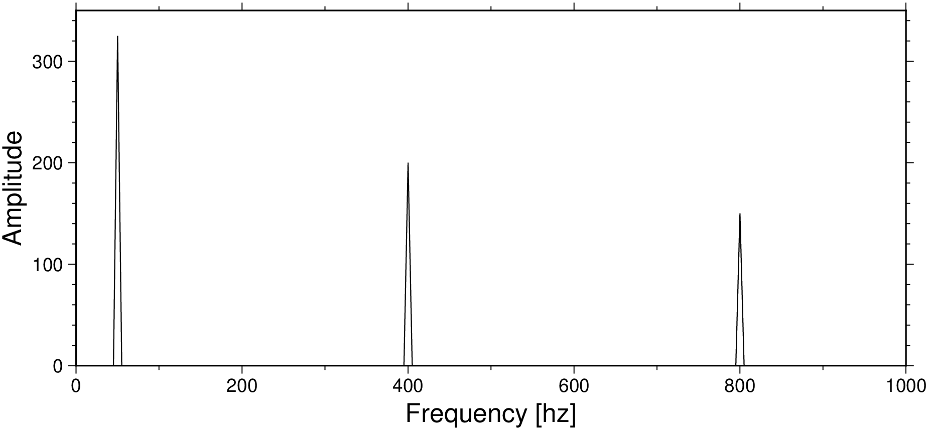
While in this simple example we can visually see that the peaks corresponds to the frequencies of the three sine waves that we generated (sig1, sig2 and sig3), let us find that numerically using the function findpeaks that we used in the autocorrelation example.

# Find the peaks in `P` but only those with a height of at least 10 to avoid the noise.
ind = findpeaks(P, min_height=10.0, xsorted=true)

6-element Vector{Int64}:
   11
   81
  161
 9841
 9921
 9991

We found 6 peaks instead of 3 because the FFT is symetrical around the center frequency (Fs / 2) and the peaks at 9991, 9921 and 9841 are the same as the peaks at 11, 81 and 161 (exercise, confirm that).

# Print frequencies of the first 3 peaks.
f[[11,81,161]]

Let's now see how we can use the FFT transformed signal to filter some of the frequencies. First we remove only the highest frequency. Since that highest frequency is at position after 81 of the FFT transformed signal, we can simply remove it by setting to zero all elements > 100.

Yfilt = copy(Y);
Yfilt[100:end] .= 0;
inv = ifft(Yfilt);
viz(real(inv), figsize=(14,6))

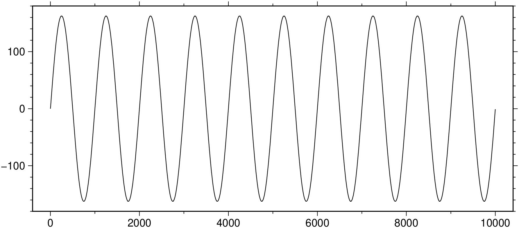
And if we want to retain only the lowest frequency component, we remove everything above 11'th element

Yfilt = copy(Y);
Yfilt[20:end] .= 0;
inv = ifft(Yfilt);
viz(real(inv), figsize=(14,6))

Exercise: remove only the lowest frequency.