gravmag3d

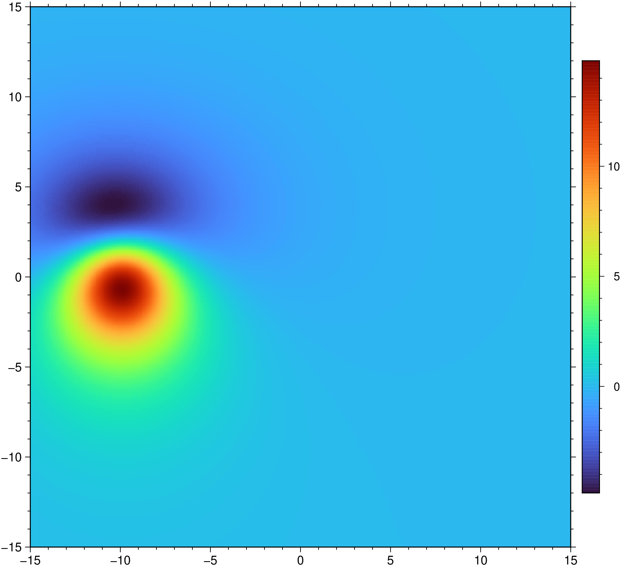
gravmag3d(fname::String="", arg1=nothing, kwargs...)

Description

Compute the gravity or magnetic anomaly of a body described by a set of triangles. The output can either be along a given set of xy locations or on a grid. This method is not particularly fast but allows computing the anomaly of arbitrarily complex shapes.

Required Arguments (not all)

• fname : Optional positional argument with the name of a xyz... file that can be read by gmtread. The xyz file can have 3, 4, 5, 6 or 8 columns. In first case (3 columns) the magnetization (or density) are assumed constant (controlled by density or mag_params). Following cases are: 4 columns -> 4rth col magnetization intensity; 5 columns: mag, mag dip; 6 columns: mag, mag dec, mag dip; 8 columns: field dec, field dip, mag, mag dec, mag dip. When n columns > 3 the third argument of the mag_params option is ignored.

• arg1 : In alternative to fname pass in a Mx3 matrix or a GMTdataset with at least 3 columns. arg1 can also be a GMTfv type like those produced by the solids functions (sphere, etc) but it must be one made of triangles. That is, the output of cube wont work because the body is made out of quadrangles. Note, if the body option is used neither this option nor fname are used.

• C or density : – density=??
  Sets body density in SI. Append either a constant, the name of a grid file or a GMTgrid grid with variable densities. This option is mutually exclusive with mag_params

• H or mag_params : – magparams=fdec/fdip/mint/mdec/mdip
  Sets parameters for computing a magnetic anomaly. Use f_dec/f_dip to set the geomagnetic declination/inclination in degrees. m_int/m_dec/m_dip are the body magnetic intensity declination and inclination.

• F or track : – track=xy_loc
  Provide xy_loc (file name or GMTdataset) locations where the anomaly will be computed. Note, this option is mutually exclusive with the save option.

• G or save or outgrid or outfile : – save=file_name.grd
  Write one or more fields directly to grids on disk or return them to the Julia REPL as grid objects. If more than one field is specified via fields then file_name must contain the format flag %s so that we can embed the field code in the file names.

• M or body : – body=shape,params | body=(shape=name, params=...)
  (An alternative to raw_triang and stl). Create geometric bodies and compute their grav/mag effect. Select among one or more of the following bodies, where x0 & y0 represent the horizontal coordinates of the body center [default to 0,0 positive up], npts is the number of points that a circle is discretized and n_slices apply when bodies are made by a pile of slices. For example Spheres and Ellipsoids are made of 2 x n_slices and Bells have n_slices [Default 5]. It is also possible to select more than one body. For example body=((shape=:prism, params="1/1/1/-5/-10/1"), (shape=:sphere, params="1/-5")) computes the effect of a prism and a sphere. Unfortunately there is no current way of selecting distinct densities or magnetic parameters for each body.

  - *bell,height/sx/sy/z0[/x0/y0/n_sig/npts/n_slices]* Gaussian of height *height* with characteristic
     STDs *sx* and *sy*. The base width (at depth *z0*) is controlled by the number of sigmas (*n_sig*) [Default = 2]
  
  - *cylinder,rad/height/z0[/x0/y0/npts/n_slices]* Cylinder of radius *rad* and height *height* and base at depth *z0*
  
  - *cone,semi_x/semi_y/height/z0[/x0/y0/npts]* Cone of semi axes *semi_x/semi_y* height *height* and base at depth *z0*
  
  - *ellipsoid,semi_x/semi_y/semi_z/z_center[/x0/y0/npts/n_slices]* Ellipsoid of semi axes *semi_x/semi_y/semi_z*
     and center depth *z_center*
  
  - *prism,side_x/side_y/side_z/z0[/x0/y0]* Prism of sides *x/y/z* and base at depth *z0*
  
  - *pyramid,side_x/side_y/height/z0[/x0/y0]* Pyramid of sides *x/y* height *height* and base at depth *z0*
  
  - *sphere,rad/z_center[/x0/y0/npts/n_slices]* Sphere of radius *rad* and center at depth *z_center*

• R or region or limits : – limits=(xmin, xmax, ymin, ymax) | limits=(BB=(xmin, xmax, ymin, ymax),) | limits=(LLUR=(xmin, xmax, ymin, ymax),units="unit") | ...more
  Specify the region of interest. More at limits. For perspective view view, optionally add zmin,zmax. This option may be used to indicate the range used for the 3-D axes. You may ask for a larger w/e/s/n region to have more room between the image and the axes.

• Tv or index : – index=vert_file | index=D
  Gives name of a vertex file defining a closed surface. The file formats correspond to the output of the triangulate module. The form raw_triang=D means that we can also pass the data as a GMTdataset

• Tr or raw_triang : – rawtriang=rawfile | raw_triang=D
  A raw format is a file with N rows (one per triangle) and 9 columns corresponding to the x, y, z coordinates of each of the three vertex of each triangle. The form raw_triang=D means that we can also pass the data as a GMTdataset

• Ts or stl or STL : – stl=raw_file
  Alternatively, the stl option indicates that the surface file is in the ASCII STL (Stereo Lithographic) format. These two type of files are used to provide a closed surface.

• noswap or no_swap : – noswap=true
  The closed surface formats (STL or raw) are assumed to be provided with the facets (triangles) following the counter-clockwise order. If that is not the case, i.e. they are clockwise oriented, use this option to bring them to the expected order. However, this order may not be easy to check. In case of doubt, compute the gravity anomaly caused by the body and see if it has the expected signal.

Optional Arguments

• E or thickness : – thickness=??
  Give layer thickness in m [Default = 0 m]. Use this option only when the triangles describe a non-closed surface and you want the anomaly of a constant thickness layer.

• L or z_obs or observation_level : – – z_obs=0
  sets level of observation [Default = 0]. That is the height (z) at which anomalies are computed.

• S or radius : – radius=30
  Set search radius in km (valid only in the two grids mode OR when thickness) [Default = 30 km]. This option serves to speed up the computation by not computing the effect of prisms that are further away than radius from the current node.

• V or verbose : – verbose=true | verbose=level
  Select verbosity level. More at verbose

Z or level or reference_level : – level=0
level of reference plane [Default = 0]. Use this option when the triangles describe a non-closed surface and the volume is defined from each triangle and this reference level. An example will be the water depth to compute a Bouguer anomaly.

Q or onebased or one_based : – onebased=true
Use this option if the indices in file (index) is 1-based instead of the default (C) 0-based. This option is needed when indices are 1-based, as likely is the case when bodies may have been created in Julia.

• f or colinfo : – colinfo=??
  Specify the data types of input and/or output columns (time or geographical data). More at

Geographic grids (dimensions of longitude, latitude) will be converted to meters via a "Flat Earth" approximation using the current ellipsoid parameters.

• h or header : – header=??
  Specify that input and/or output file(s) have n header records. More at

• i or incol or incols : – incol=col_num | incol="opts"
  Select input columns and transformations (0 is first column, t is trailing text, append word to read one word only). More at incol

• o or outcol : – outcol=??
  Select specific data columns for primary output, in arbitrary order. More at

• r or reg or registration : – reg=:p | reg=:g
  Select gridline or pixel node registration. Used only when output is a grid. More at

Grid Distance Units

If the grid does not have meter as the horizontal unit, append +u\unit to the input file name to convert from the specified unit to meter. If your grid is geographic, convert distances to meters by supplying f=:g instead.

Example

To compute the magnetic anomaly of a cube of unit sides located at 5 meters depth and centered at -10,1 in a domain R="-15/15/-15/15" with a magnetization of 10 Am with a declination of 10 degrees, inclination of 60 in a magnetic field with -10 deg of declination and 40 deg of inclination, do:

using GMT

G = gravmag3d(region="-15/15/-15/15", I=0.1, mag_params="10/60/10/-10/40", body=(shape=:prism, params="1/1/1/-5/-10/1"));
viz(G, colorbar=true)

See Also

grdgravmag3d, gravprisms, talwani2d, talwani3d, triangulate

Reference

Okabe, M., 1979, Analytical expressions for gravity anomalies due to polyhedral bodies and translation into magnetic anomalies, Geophysics, 44, 730-741.