(7) A simple location map

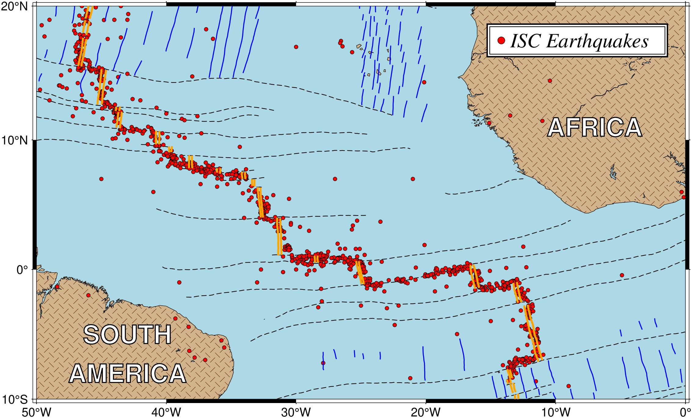
Many scientific papers start out by showing a location map of the region of interest. This map will typically also contain certain features and labels. This example will present a location map for the equatorial Atlantic ocean, where fracture zones and mid-ocean ridge segments have been plotted. We also would like to plot earthquake locations and available isochrons. We have obtained one file, quakes_07.txt, which contains the position and magnitude of available earthquakes in the region. We choose to use magnitude/40 for the symbol-size in cm. The digital fracture zone traces (fz_07.txt) and isochrons (0 isochron as ridge_07.txt, the rest as isochron_07.txt) were digitized from available maps 1. We create the final location map with the following script:

using GMT

coast(region=(-50,0,-10,20), water=:lightblue, land="P300/26:FtanBdarkbrown",
      res=:low, shore=:thinnest, frame=(annot=10,), proj=:Mercator, figsize=18,
      par=(:FORMAT_GEO_MAP, :dddF))
plot!("@fz_07.txt", pen="thinner,-")
scatter!("@quakes_07.txt", h=1, i="0,1,2s0.01", marker=:circle, fill=:red,
         markerline=:thinnest, MarkerSize="3p")
plot!("@isochron_07.txt", pen="thin,blue")
plot!("@ridge_07.txt", pen=(:thicker,:orange))
legend!(mat2ds("S 0.25 c 0.2 red thinnest 0.5 ISC Earthquakes"),
        pos=(inside=true, anchor=:TR, width=5.0, offset=0.5),
        box=(pen=:thick,inner=:thinner,fill=:white),
        par=(:FONT_ANNOT_PRIMARY, "16p,Times-Italic"))
text!(mat2ds([-43 -5; -43 -8; -7 11], ["SOUTH", "AMERICA", "AFRICA"]),
      font=(20,"Helvetica-Bold","white=thin"), show=true)