using GMT, Printf
resetGMT() # hide
# Interpolate data of Mars radius from Mariner9 and Viking Orbiter spacecrafts
makecpt(cmap=:rainbow, range=(-7000,15000))
centroid = gmtspatial("@GSHHS_h_Australia.txt", colinfo=:g, length=:k)
basemap(region=(112,154,-40,-10), proj=:Merc, figsize=14, frame=(axes=:WSne, annot=20, bg=[240,255,240]))
plot!("@GSHHS_h_Australia.txt", pen=:faint, fill=(240,255,240))
plot!("@GSHHS_h_Australia.txt", ms=0.025, fill=:red)
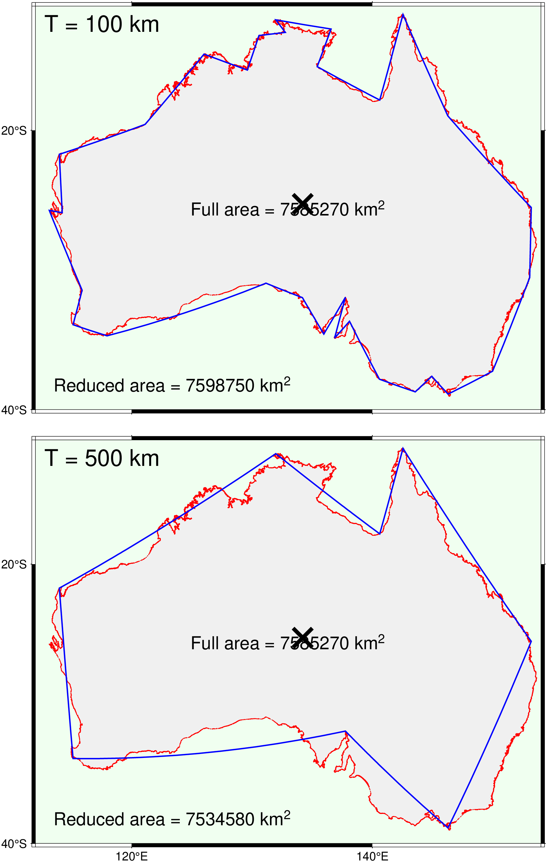
T500k = gmtsimplify("@GSHHS_h_Australia.txt", tolerance="500k");
t = gmtspatial("@GSHHS_h_Australia.txt", colinfo=:g, length=:k);
area = @sprintf("Full area = %.0f km@+2@+", t.data[3]);
t = gmtspatial(T500k, colinfo=:g, length=:k);
area_T500k = @sprintf("Reduced area = %.0f km@+2@+", t.data[3]);
plot!(T500k, pen=(1,:blue))
plot!(centroid, marker=:cross, ms=0.75, ml=3)
text!(text_record([112 -10], "T = 500 km"), offset=(away=true, shift=(0.25,0.25)), font=18, justify=:TL)
text!(text_record(area), font=14, region_justify=:CM)
text!(text_record(area_T500k), font=14, region_justify=:LB, offset=(away=true, shift=0.5))
basemap!(frame=(axes=:Wsne, annot=20, bg=[240,255,240]), yshift=12)
plot!("@GSHHS_h_Australia.txt", pen=:faint, fill=(240,255,240))
plot!("@GSHHS_h_Australia.txt", ms=0.025, fill=:red)
T100k = gmtsimplify("@GSHHS_h_Australia.txt", tolerance="100k");
t = gmtspatial(T100k, colinfo=:g, length=:k);
area_T100k = @sprintf("Reduced area = %.0f km@+2@+", t.data[3]);
plot!(T100k, pen=(1,:blue))
plot!(centroid, marker=:cross, ms=0.75, ml=3)
text!(text_record([112 -10], "T = 100 km"), offset=(away=true, shift=(0.25,0.25)), font=18, justify=:TL)
text!(text_record(area), font=14, region_justify=:CM)
text!(text_record(area_T100k), font=14, region_justify=:LB, offset=(away=true, shift=0.5), show=true)