using GMT, DataFrames, CSV[ Info: Precompiling GMTDataFramesExt [b0121151-b40e-578b-8798-214dacfa5da6]
A choropleth is a thematic map where areas are colored in proportion to a variable such as population density. GMT lets us plot choropleth maps but the process is not straightforward because we need to put the color information in the header of a multi-segment file. To facilitate this, some tools were added to the Julia wrapper.
(But see also the more extended example in [tutorials])
Load packages needed to download data and put into a DataFrame
using GMT, DataFrames, CSV[ Info: Precompiling GMTDataFramesExt [b0121151-b40e-578b-8798-214dacfa5da6]
paises = CSV.File(HTTP.get("https://raw.githubusercontent.com/tillnagel/unfolding/master/data/data/countries-population-density.csv").body, delim=';') |> DataFrame;Extract the Europe countries from the DCW file
eu = coast(DCW="=EU+z", dump=true);Generate two vector with country codes (2 chars codes) and the population density for European countries.
codes, vals = GMT.mk_codes_values(paises[!, 2], paises[!, 3], region="eu");Create a Categorical CPT that allows plotting the choropleth. Note that we need to limit the CPT range to leave out the very high density states like Monaco otherwise all others would get the same color.
C = cpt4dcw(codes, vals, range=[10, 500, 10]);Show the result
plot(eu, cmap=C, fill="+z", proj=:guess, R="-76/36/26/84", title="Population density",
    colorbar=true, show=true)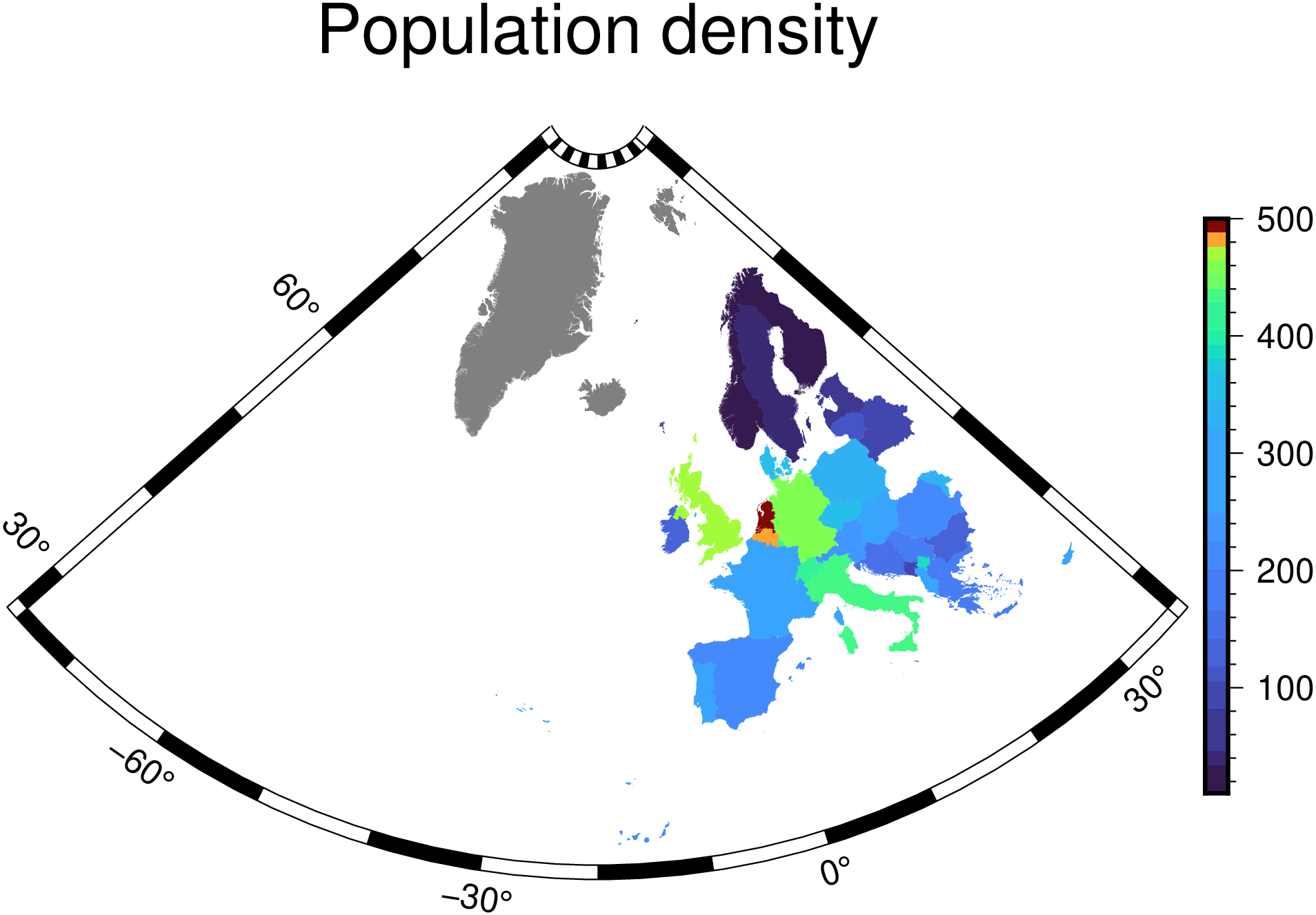
While GMT come with the world countries in its DCW data base, those countries polygons have a somewhat too high resolution for world maps and hence produce files unnecessarily, which also makes them slower to create. An alternative is to use a much lower resolution file that can be found here but whose download link is here. And we can read it directly into GMT (and wait a bit while it gets downloaded).
countries = gmtread("/vsicurl/https://github.com/datasets/geo-countries/raw/main/data/countries.geojson");The country polygons have attributes like:
Attributes: Dict("ISO_A2" => "AW", "ISO_A3" => "ABW", "ADMIN" => "Aruba")
Like in the Europe case above, we load the world population into a DataFrame
pop = CSV.File(HTTP.get("https://raw.githubusercontent.com/tillnagel/unfolding/master/data/data/countries-population-density.csv").body, delim=';') |> DataFrame;The contents of that file look like this:
julia> pop
248×3 DataFrame
 Row │ Country Name                       Country Code  2010
     │ String                             String3       Float64?
─────┼───────────────────────────────────────────────────────────
   1 │ Arab World                         ARB            26.2725
   2 │ Caribbean small states             CSS            16.9939
   3 │ East Asia & Pacific (all income …  EAS            90.5122
2 │ Caribbean small states CSS 16.9939 3 │ East Asia & Pacific (all income … EAS 90.5122
So we must now link the countries in `countries` with density in `2010` via the attribute `ISO_A3` in `countries`
and the third column in `pop`. To make a global choropleth map with the population density we will use first the
polygonlevels function to get as the population density in the same order as the country polygons are
stored in the `countries` GMTdataset.

```julia
zvals = polygonlevels(countries, string.(pop[!,2]), pop[!,3], att="ISO_A3");
And now we are ready to make the map
# First create the colormap. Limit the maximum range to 500 otherwise states
# like Monaco would the all the `reds` and the rest of the world would be all blues.
C = makecpt(range=(0,500,10));
plot(countries, region=(-180,180,-60,85), level=zvals, cmap=C, proj=:guess,
     title="World population density", colorbar=true, show=true)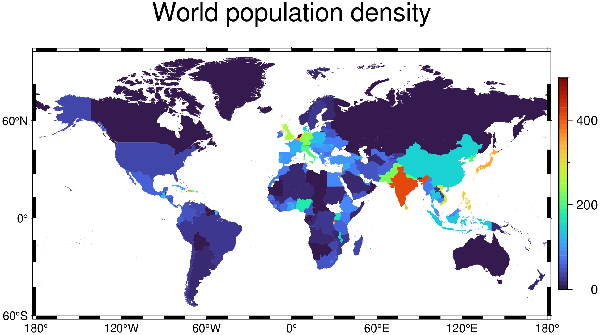
First, download the Portuguese district polygons shape file from this Github repo Next load it with:
using GMT, DataFrames, CSV

Pt = gmtread("C:\\programs\\compa_libs\\covid19pt\\extra\\mapas\\concelhos\\concelhos.shp");
Download and load a CSV file from same repo with rate of infection per district. Load it into a DataFrame to simplify data extraction.
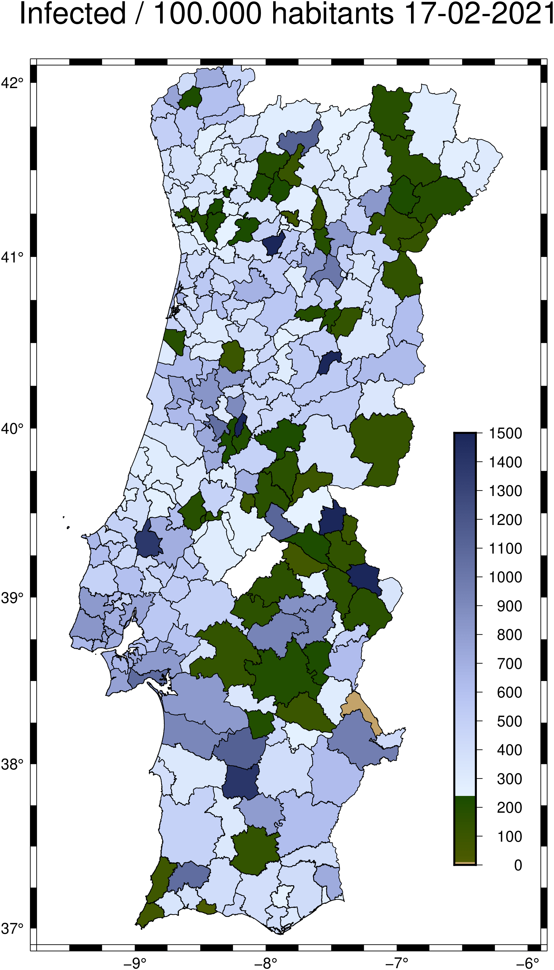
incidence = CSV.read("C:\\programs\\compa_libs\\covid19pt\\data_concelhos_incidencia.csv", DataFrame);Get the rate of incidence in number of infected per 100_000 habitants for the last reported week.
r = collect(incidence[end, 2:end]);But the damn polygon names above are all uppercase, Ghrrr. We will have to take care of that.
ids = names(incidence)[2:end];Each of the Pt datasets have attributes (e.g., Pt[1].attrib) and the one that is common with the names in ids is the Pt[1].attrib["NAME2"] (the conselho name). But the names in dataconcelhosincidencia.csv (from which the ids are derived) and the concelhos.shp (that we read into Pt) do not use the same case (one is full upper case) so we need to use the nocase=true below. The comparison is made inside the next call to the polygonlevels() function that takes care to return the numerical vector that we need in plot’s level option.
zvals = polygonlevels(Pt, ids, r, att="NAME_2", nocase=true);Create a Colormap to paint the district polygons
C = makecpt(range=(0,1500,10), inverse=true, cmap=:oleron, hinge=240, bg=:o);Get the date for the data being represented to use in title
date = incidence[end,1];And finaly do the plot
plot(Pt, level=zvals, cmap=C, pen=0.5, region=(-9.75,-5.9,36.9,42.1), proj=:Mercator,
     title="Infected / 100.000 habitants " * date)

colorbar!(pos=(anchor=:MR,length=(12,0.6), offset=(-2.4,-4)), color=C,
          axes=(annot=100,), show=true)