using GMT
D = gmtsimplify("@GSHHS_h_Australia.txt", tolerance="100k")
plot("@GSHHS_h_Australia.txt", plot=(data=D, lc=:red), show=true)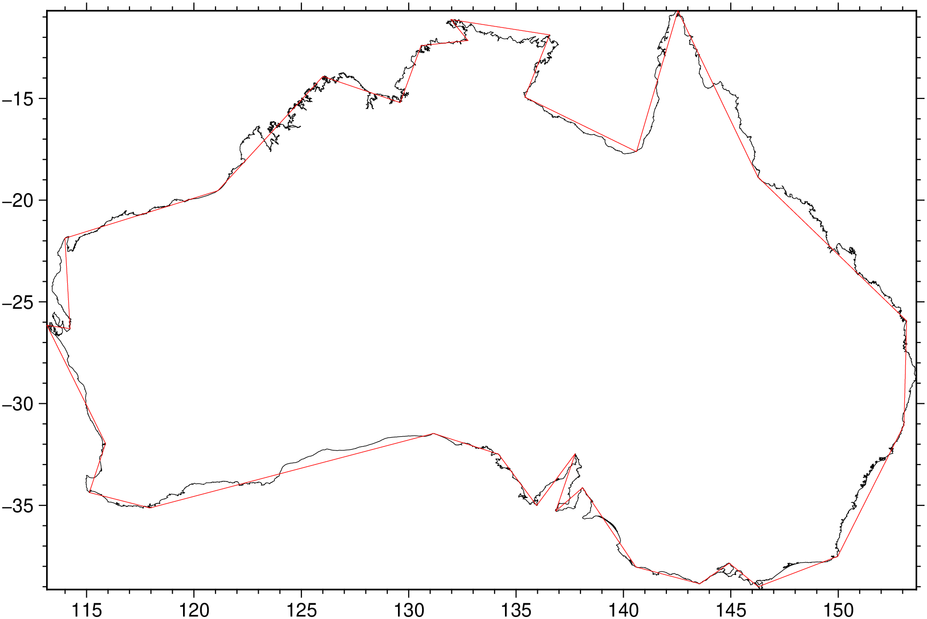
gmtsimplify(cmd0::String="", arg1=nothing; kwargs...)Line reduction using the Douglas-Peucker algorithm
simplify reads one or more data files and apply the Douglas-Peucker line simplification algorithm. The method recursively subdivides a polygon until a run of points can be replaced by a straight line segment, with no point in that run deviating from the straight line by more than the tolerance. Have a look at this site to get a visual insight on how the algorithm works (https://en.wikipedia.org/wiki/Ramer–Douglas–Peucker_algorithm)
-T or tol or tolerance : – tolerance=tol
Specifies the maximum mismatch tolerance in the user units. If the data are not Cartesian then append a suitable distance unit (see [Units]).
V or verbose : – verbose=true | verbose=level
Select verbosity level. More at verbose
bi or binary_in : – binary_in=??
Select native binary format for primary table input. More at
bo or binary_out : – binary_out=??
Select native binary format for table output. More at
di or nodata_in : – nodata_in=??
Substitute specific values with NaN. More at
e or pattern : – pattern=??
Only accept ASCII data records that contain the specified pattern. More at
f or colinfo : – colinfo=??
Specify the data types of input and/or output columns (time or geographical data). More at
g or gap : – gap=??
Examine the spacing between consecutive data points in order to impose breaks in the line. More at
h or header : – header=??
Specify that input and/or output file(s) have n header records. More at
i or incol or incols : – incol=col_num | incol=“opts”
Select input columns and transformations (0 is first column, t is trailing text, append word to read one word only). More at incol
o or outcol : – outcol=??
Select specific data columns for primary output, in arbitrary order. More at
q or inrows : – inrows=??
Select specific data rows to be read and/or written. More at
yx : – yx=true
Swap 1st and 2nd column on input and/or output. More at
Units
For map distance unit, append unit d for arc degree, m for arc minute, and s for arc second, or e for meter [Default unless stated otherwise], f for foot, k for km, M for statute mile, n for nautical mile, and u for US survey foot. By default we compute such distances using a spherical approximation with great circles (-jg) using the authalic radius (see PROJ_MEAN_RADIUS). You can use -jf to perform “Flat Earth” calculations (quicker but less accurate) or -je to perform exact geodesic calculations (slower but more accurate; see PROJ_GEODESIC for method used).
To reduce the remote high-resolution GSHHG polygon for Australia down to a tolerance of 500 km, use:
using GMT
D = gmtsimplify("@GSHHS_h_Australia.txt", tolerance="100k")
plot("@GSHHS_h_Australia.txt", plot=(data=D, lc=:red), show=true)
To reduce the Cartesian lines xylines.txt using a tolerance of 0.45 and write the reduced lines to file new_xylines.txt, run:
D = gmtsimplify("xylines.txt", tol=0.45)There is a slight difference in how simplify processes lines versus closed polygons. Segments that are explicitly closed will be considered polygons, otherwise we treat them as line segments. Hence, segments recognized as polygons may reduce to a 3-point polygon with no area; these are suppressed from the output.
One known issue with the Douglas-Peucker has to do with crossovers. Specifically, it cannot be guaranteed that the reduced line does not cross itself. Depending on how many lines you are considering it is also possible that reduced lines may intersect other reduced lines. Finally, the current implementation only does Flat Earth calculations even if you specify spherical; simplify will issue a warning and reset the calculation mode to Flat Earth.
Douglas, D. H., and T. K. Peucker, Algorithms for the reduction of the number of points required to represent a digitized line of its caricature, Can. Cartogr., 10, 112-122, 1973.
This implementation of the algorithm has been kindly provided by Dr. Gary J. Robinson, Department of Meteorology, University of Reading, Reading, UK; his subroutine forms the basis for this program.
This function has multiple methods:
gmtsimplify(cmd0::String; kwargs...) - gmtsimplify.jl:28gmtsimplify(arg1; kwargs...) - gmtsimplify.jl:29