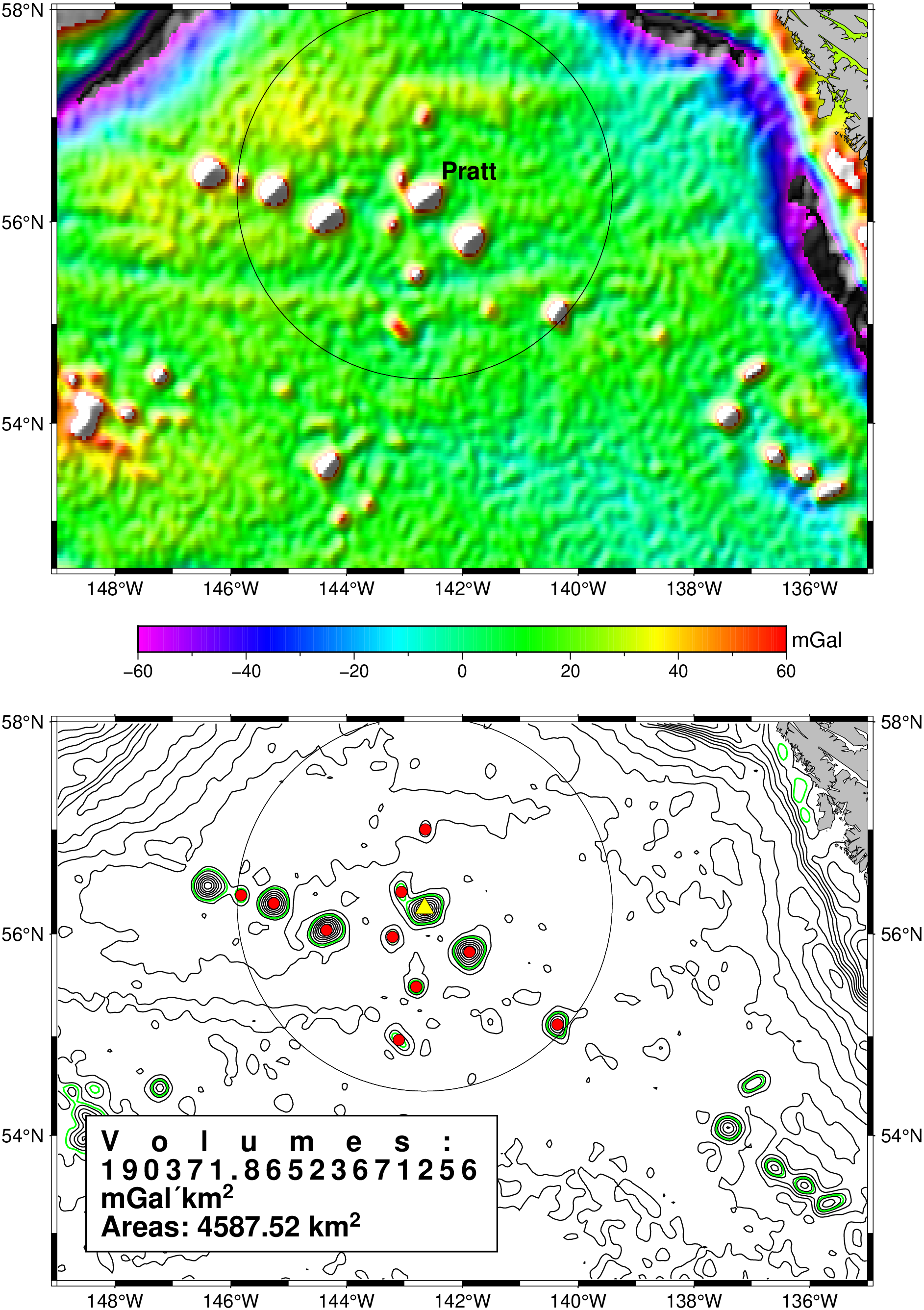
using GMT, Printf

pratt = [-142.65 56.25 400]

# First generate gravity image w/ shading, label Pratt, and draw a circle
# of radius = 200 km centered on Pratt.
grav_cpt = makecpt(color=:rainbow, range=(-60,60));
grdimage("@AK_gulf_grav.nc", shade=:default, frame=(annot=2,ticks=1), proj=:merc, figsize=14, xshift=3.8, yshift=14.9)
coast!(region="@AK_gulf_grav.nc", land=:gray, shore=:thinnest)
colorbar!(pos=(anchor=:BC, offset=(0,1)), xaxis=(annot=20, ticks=10), ylabel="mGal")
text!(text_record(pratt, "Pratt"), font=(12,"Helvetica-Bold"), justify=:LB, offset="8p")
plot!(pratt, marker="E-", markerline=:thinnest)

# Then draw 10 mGal contours and overlay 50 mGal contour in green
grdcontour!("@AK_gulf_grav.nc", cont=20, frame=(axes=:WSEn, annot=2, ticks=1), yshift=-12.3)
# Save 50 mGal contours to individual files, then plot them
grdcontour!("@AK_gulf_grav.nc", cont=10, range=(49,51), dump="sm_%c.txt")
plot!("sm_C.txt", lw=:thin, lc=:green)
coast!(land=:gray, shore=:thinnest)
plot!(pratt, marker="E-", markerline=:thinnest)

# Now determine centers of each enclosed seamount > 50 mGal but only plot
# the ones within 200 km of Pratt seamount.

# First determine mean location of each closed contour and add it to the file centers.txt
centers = gmtspatial("sm_C.txt", length=true, colinfo=:g)

# Only plot the ones within 200 km
t = gmtselect(centers, C=(pratt,"200k"), colinfo=:g)
plot!(t, marker=:Circle, ms=0.2, mc=:red, MarkerLine=:thinnest)
plot!(pratt, marker=:Triangle, ms=0.25, fill=:yellow, MarkerLine=:thinnest)

# Then report the volume and area of these seamounts only
# by masking out data outside the 200 km-radius circle
# and then evaluate area/volume for the 50 mGal contour

Gmask = gmt(string("grdmath -R@AK_gulf_grav.nc ", pratt[1], " ", pratt[2], " SDIST ="))
Gmask = grdclip(Gmask, above=(200, NaN), below=(200, 1))
Gtmp = gmt("grdmath @AK_gulf_grav.nc ? MUL =", Gmask);
av   = grdvolume(Gtmp, cont=50, unit=:k);

T = mat2ds(["Volumes: $(av.data[3]) mGal\\264km@+2@+"
    ""
    @sprintf("Areas: %.2f km@+2@+", av.data[2])], hdr="> -149 52.5 14p 2.6i j")

text!(T, paragraph=true, fill=:white, pen=:thin, offset=0.75, font=(14,"Helvetica-Bold"),
      justify=:LB, clearance=0.25, show=true)