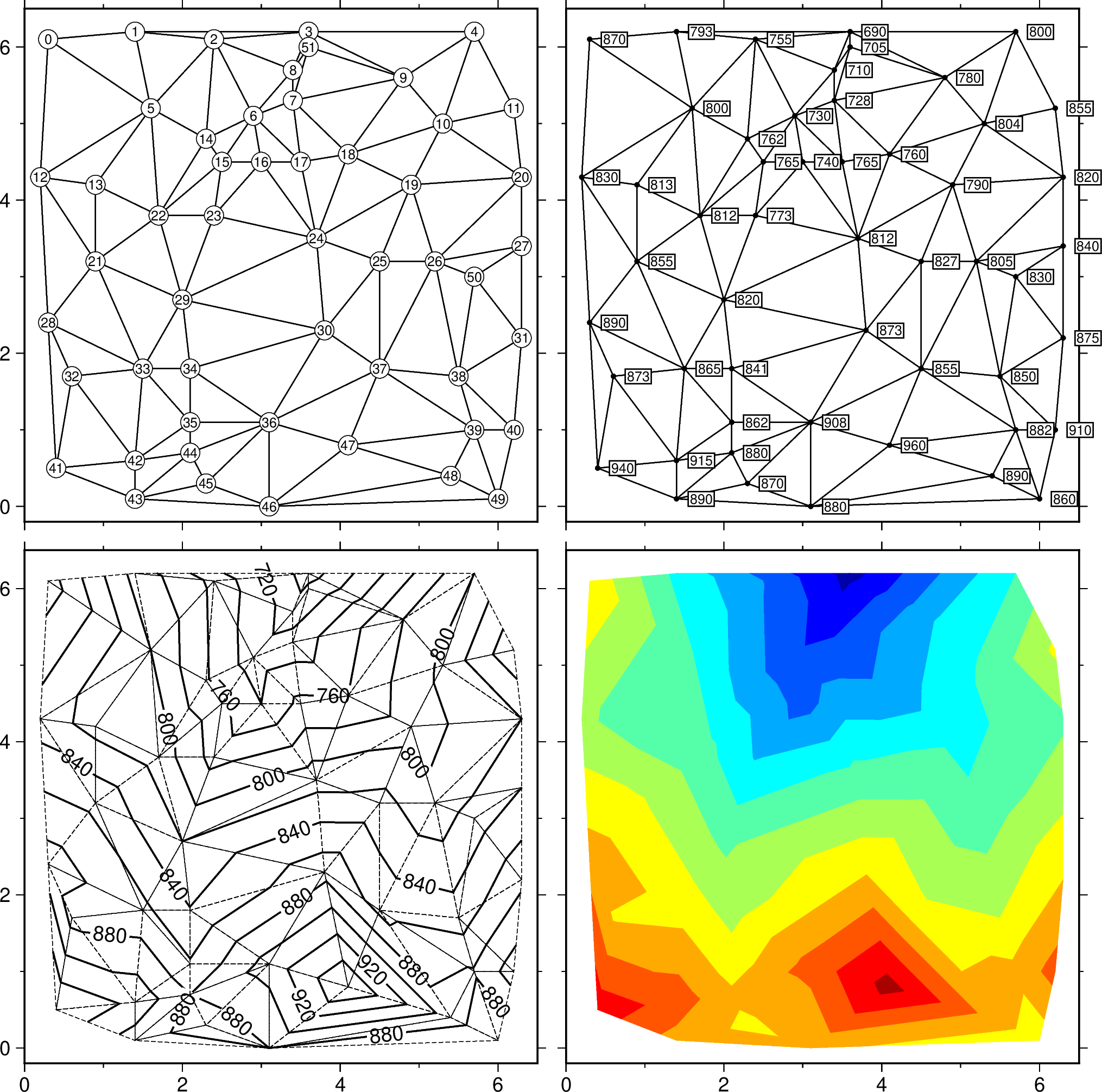
using GMT

table_5 = gmtread("@Table_5_11.txt")    # The data used in this example
T = gmtinfo(table_5, nearest_multiple=(dz=25, col=2))
makecpt(color=:jet, range=T.text[1][3:end])  # Make it also the current cmap

subplot(grid=(2,2), limits=(0,6.5,-0.2,6.5), col_axes=(bott=true,), row_axes=(left=true,),
        figsize=8, margins=0.1, panel_size=(8,0), tite="Delaunay Triangulation")
    # First draw network and label the nodes
    net_xy = triangulate(table_5, M=true)
    plot(net_xy, lw=:thinner)
    plot(table_5, marker=:circle, ms=0.3, fill=:white, MarkerLine=:thinnest)
    text(table_5, font=6, rec_number=0)

    # Then draw network and print the node values
    plot(net_xy, lw=:thinner, panel=(1,2))
    plot(table_5, marker=:circle, ms=0.08, fill=:black)
    text(table_5, zvalues=true, font=6, justify=:LM, fill=:white, pen="", clearance="1p", offset=("6p",0), noclip=true)

    # Finally color the topography
    contour(table_5, pen=:thin, mesh=(:thinnest,:dashed), labels=(dist=2.5,), panel=(2,1))
    contour(table_5, colorize=true, panel=(2,2))
subplot("show")