(27) Plotting Sandwell/Smith Mercator img grids
Next, we show how to plot a data grid that is distributed in projected form. The gravity and predicted bathymetry grids produced by David Sandwell and Walter H. F. Smith are not geographical grids but instead given on a spherical Mercator grid. The GMT supplement imgsrc has tools to extract subsets of these large grids. If you need to make a non-Mercator map then you must extract a geographic grid using $img2grd$ and then plot it using your desired map projection. However, if you want to make a Mercator map then you can save time and preserve data quality by avoiding to re-project the data set twice since it is already in a Mercator projection. This example shows how this is accomplished. We have used the -M option in img2grd 1 to pull out the grid in Mercator units (i.e., do not invert the Mercator projection) and then simply plot this remote grid using a linear projection with a suitable scale (here 0.25 inches per degrees of longitude). To overlay basemaps and features that has geographic longitude/latitude coordinates we must remember two key issues:
- This is a spherical Mercator grid so we must use ``par=(PROJ_ELLIPSOID=:Sphere,)`` with all commands that involve projections (or use gmtset to change the setting). - Select Mercator projection and use the same scale that was used with the linear projection.
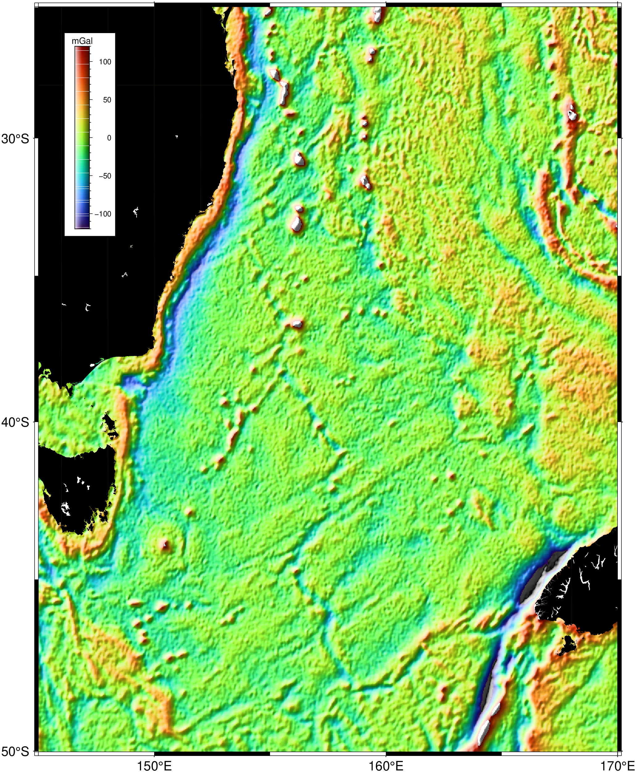
This map of the Tasman Sea shows the marine gravity anomalies with land painted black. A color scale bar was then added to complete the illustration.
using GMT

# Gravity in tasman_grav.nc is in 0.1 mGal increments and the grid
# is already in projected Mercator x/y units.

# Make a suitable cpt file for mGal
grav_cpt = makecpt(range=(-120,120))

# Since this is a Mercator grid we use a linear projection
grdimage("@tasman_grav.nc=ns+s0.1", frame=:none, shade=:default, figscale=0.635)

# Then use gmt pscoast to plot land; get original -R from grid remark
# and use Mercator gmt projection with same scale as above on a spherical Earth
R = grdinfo("@tasman_grav.nc", nearest=:i)
R = R.text[1][3:end]
coast!(region=R, proj=:merc, figscale=0.635, frame=(axes=:WSne, annot=10, ticks=5),
       land=:black, river_fill=:white, res=:high,
       par=(FORMAT_GEO_MAP="dddF", PROJ_ELLIPSOID=:Sphere))

# Put a color legend in top-left corner of the land mask
colorbar!(region=R, pos=(inside=true, anchor=:TL, offset=1, length=(5, 0.4)),
          xaxis=(annot=50, ticks=10), ylabel="mGal", shade=true, box=(pen=1, fill=:white), show=true)
These docs were autogenerated using GMT: v1.33.1