parkermag

G = parkermag(mag, bat, dir::String="dir"; year=2020.0, nnx=0, nny=0, nterms=6, zobs=0.0,
              wshort=0.0, wlong=0.0, slin=0.0, sdip=0.0, sdec=0.0, thickness=0.5, pct=30,
              geocentric=false, padtype::String="taper", isRTP=false, verbose=false)::GMTgrid

Calculate the magnetic direct or inverse problem using Parker's [1973] Fourier series summation approach.

Depending on the vaule of dir it will calculate the direct or inverse problem. The direct problem calculates magnetic field given a magnetization and bathymetry. The inverse calculates magnetization from magnetic field and bathymetry.

This function is an adaptation of the Mirone code that itself was an adaptation of Maurice Tivey's code MATLAB Version from 1992.

Args

• mag: GMTgrid or filename of the magnetic field (nT) for the direct problem or magnetization (A/m) for the inverse problem.

• bat: bathymetry grid (km positive up)

• dir: "dir" for direct problem or "inv" for inverse problem.

Kwargs

• year: year of observation in decimal years.

• nnx, nny: suitable grid dimensions for FFT. By default they are calculated as the next good FFT number that is 30% larger than the size of the input grids. But this value can be set via the pct option. To the list of the good FFT numbers run this command: gmt("grdfft -Ns")

• nterms: number of terms in the Parker summation (default is 6)

• zobs: Level of observation in km. This is zero for marine magnetics surveys.

• wshort: short wavelength cutoff (for the inverse problem only). By default we comput it automatically from

  the grid increments, but often it may require a finer tunning.

• wlong: long wavelength cutoff (for the inverse problem only). By default it is also assigned automatically as max(dx*nnx, dy*nny) with an additional condition of not being shorter than 150 km.

• slin: strike of line of observation (for the direct problem only)

• sdip: dip of line of observation. Use sdip=90 for a geocentric dipole

• sdec: declination of magnetization.

• thickness: thickness of source layer in km

• pct: percentage of grid size to augment. See also the nnx and nny options. Use pct=0 to force nnx and nny to be the same as the size of the input grids

• padtype: Strategy used when padding an array. The default is to use taper Hanning window. Alternative is zero that pads with zeros.

• isRTP: Set this to true if the field is already reduced-to-the-pole

• geocentric: use the geocentric dipole. Same as leaving sdip=0 & sdec=0

• verbose: verbose mode

Returns

A GMTgrid with the computed magnetic fiels or magnetization.

Example

A synthetic example. Make a Kaba like magnetization distribution of 10 A/m, compute the magnetic field created by it and invert this field.

using GMT, FFTW

m = zeros(Float32, 64,64);  m[32:40,32:40] .= 10;
h = fill(-2.0f0, 64,64);
Gm = mat2grid(m, hdr=[30., 30.32, 30., 30.32]);
Gh = mat2grid(h, hdr=[30., 30.32, 30., 30.32]);
f3d = parkermag(Gm,  Gh, "dir", year=2000, thickness=1, pct=0);
m3d = parkermag(f3d, Gh, "inv", year=2000, thickness=1, pct=0);

grdimage(f3d, figsize=6, title="Field (nT)", colorbar=true)
grdview!(m3d, figsize=6, zsize=4, view=(210, 40), title="Magnetization (A/m)", cmap=:auto, surf=:image, B=:za, xshift=8, show=true)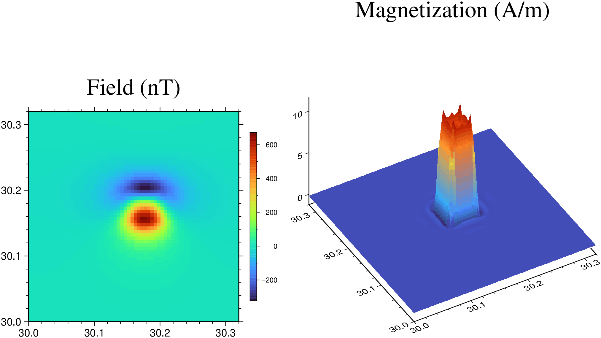

See Also

parkergrav, gravfft