ternary

ternary(cmd0::String="", arg1=[]; kwargs...)

keywords: GMT, Julia, ternary plots

Plot data on ternary diagrams

Description

Reads (a, b, c [, z]) records from table and plots symbols at those locations on a ternary diagram. If a symbol is selected and no symbol size given, then we will interpret the fourth column of the input data as symbol size. Symbols whose size is <= 0 are skipped. If no symbols are specified then the symbol code (see marker below) must be present as last column in the input. If marker is not specified then we instead plot lines or polygons.

Parameters

• B or axes or frame : – frame=??
  For ternary diagrams the three sides are referred to as a, b, and c. Thus, to give specific settings for one of these axis you must include the axis letter before the arguments. If all axes have the same arguments then only give one option without the axis letter. For more details, see the example at the bottom of this page and the general frame docs.

• C or color or cmap : – color=cpt
  Give a CPT or specify color="color1,color2 [,color3 ,...]" or color=((r1,g1,b1),(r2,g2,b2),...) to build a linear continuous CPT from those colors automatically, where z starts at 0 and is incremented by one for each color. In this case color_n can be a [r g b] triplet, a color name, or an HTML hexadecimal color (e.g. #aabbcc). If symbol is set, let symbol fill color be determined by the z-value in the fourth column. Additional fields are shifted over by one column (optional size would be 5th rather than 4th field, etc.).

• G or markerfacecolor or MarkerFaceColor or markercolor or mc or fill
  Select color or pattern for filling of symbols [Default is no fill]. Note that plot will search for fill and pen settings in all the segment headers (when passing a GMTdaset or file of a multi-segment dataset) and let any values thus found over-ride the command line settings (but those must be provided in the terse GMT syntax). See Setting color for extend color selection (including color map generation).

• J or proj or projection : – proj=width
  The only valid projection is linear plot with specified ternary width. Use a negative width to indicate that positive axes directions be clock-wise [Default lets the a, b, c axes be positive in a counter-clockwise direction].

• L or vertex_labels : – vertex_labels="Lab1/lab2/Lab3" | vertex_labels=("Lab1", "lab2", "Lab3")
  Set the labels for the three diagram vertices where the component is 100% [none]. These are placed a distance of three times the MAP_LABEL_OFFSET setting from their respective corners. To skip any one of then, specify that label as "-".

• M or dump : – dump=true
  Do no plot. Instead, convert the input (a, b, c [, z]) records to Cartesian (x, y, [, z]) records, where x, y are normalized coordinates on the triangle (i.e., 0–1 in x and 0–sqrt(3)/2 in y).

• N or noclip or no_clip : noclip=true
  Do NOT clip symbols that fall outside map border [Default plots points whose coordinates are strictly inside the map border only].

• R or region or limits : – limits=(xmin, xmax, ymin, ymax) | limits=(BB=(xmin, xmax, ymin, ymax),) | limits=(LLUR=(xmin, xmax, ymin, ymax),units="unit") | ...more
  Specify the region of interest. More at limits. For perspective view view, optionally add zmin,zmax. This option may be used to indicate the range used for the 3-D axes. You may ask for a larger w/e/s/n region to have more room between the image and the axes.

• S or marker or symbol : – symbol=(symb=name, size=val, unit=unity) or marker|Marker|shape=name, markersize|MarkerSize|ms|size=val
  Plot individual symbols in a ternary diagram. If marker is not given then we will instead plot lines (requires markerline) or polygons (requires cmap or fill). For details on symbols see the symbol option in plot

Other than the above options, the kwargs input accepts still the following options:

• image : – image=true
  Fills the ternary plot with an image computed automatically with grdimage from a grid interpolated with surface

• contour : – contour=??
  This option works in two different ways. If used together with image it overlays a contour by doing a call to grdcontour. However, if used alone it will call contour to do the contours. The difference is important because this option can be used in default mode with contour=true where the number and annotated contours is picked automatically, or the use can exert full control by passing as argument a NamedTuple with all options appropriated to that module. e.g. contour=(cont=10, annot=20, pen=0.5)

• contourf : – contourf=??
  Works a bit like the standalone contour. If used with contourf=true call make a filled contour using automatic parameters. The form contourf=(...) let us selects options of the contourf module.

• clockwise : – clockwise=true` Set it to true to indicate that positive axes directions be clock-wise [Default lets the a, b, c axes be positive in a counter-clockwise direction].

• U or time_stamp : – time_stamp=true | time_stamp=(just="code", pos=(dx,dy), label="label", com=true)
  Draw GMT time stamp logo on plot. More at timestamp

• V or verbose : – verbose=true | verbose=level
  Select verbosity level. More at verbose

• W or pen=pen
  Set pen attributes for the arrow stem [Defaults: width = default, color = black, style = solid]. See Pen attributes

• X or xshift or x_offset : xshift=true | xshift=x-shift | xshift=(shift=x-shift, mov="a|c|f|r")
  Shift plot origin. More at xshift

• Y or yshift or y_offset : yshift=true | yshift=y-shift | yshift=(shift=y-shift, mov="a|c|f|r")
  Shift plot origin. More at yshift

• bi or binary_in : – binary_in=??
  Select native binary format for primary table input. More at

• di or nodata_in : – nodata_in=??
  Substitute specific values with NaN. More at

• e or pattern : – pattern=??
  Only accept ASCII data records that contain the specified pattern. More at

• f or colinfo : – colinfo=??
  Specify the data types of input and/or output columns (time or geographical data). More at

• g or gap : – gap=??
  Examine the spacing between consecutive data points in order to impose breaks in the line. More at

• h or header : – header=??
  Specify that input and/or output file(s) have n header records. More at

• i or incol or incols : – incol=col_num | incol="opts"
  Select input columns and transformations (0 is first column, t is trailing text, append word to read one word only). More at incol

• q or inrows : – inrows=??
  Select specific data rows to be read and/or written. More at

• s or skiprows or skip_NaN : – skip_NaN=true | skip_NaN="<cols[+a][+r]>"
  Suppress output of data records whose z-value(s) equal NaN. More at

• yx : – yx=true
  Swap 1st and 2nd column on input and/or output. More at

• p or view or perspective : – view=(azim, elev)
  Default is viewpoint from an azimuth of 200 and elevation of 30 degrees.
  Specify the viewpoint in terms of azimuth and elevation. The azimuth is the horizontal rotation about the z-axis as measured in degrees from the positive y-axis. That is, from North. This option is not yet fully expanded. Current alternatives are:

  • view=??
    A full GMT compact string with the full set of options.

  • view=(azim,elev)
    A two elements tuple with azimuth and elevation

  • view=true
    To propagate the viewpoint used in a previous module (makes sense only in bar3!)

  More at perspective

• t or transparency or alpha: – alpha=50
  Set PDF transparency level for an overlay, in (0-100] percent range. [Default is 0, i.e., opaque]. Works only for the PDF and PNG formats.

Examples

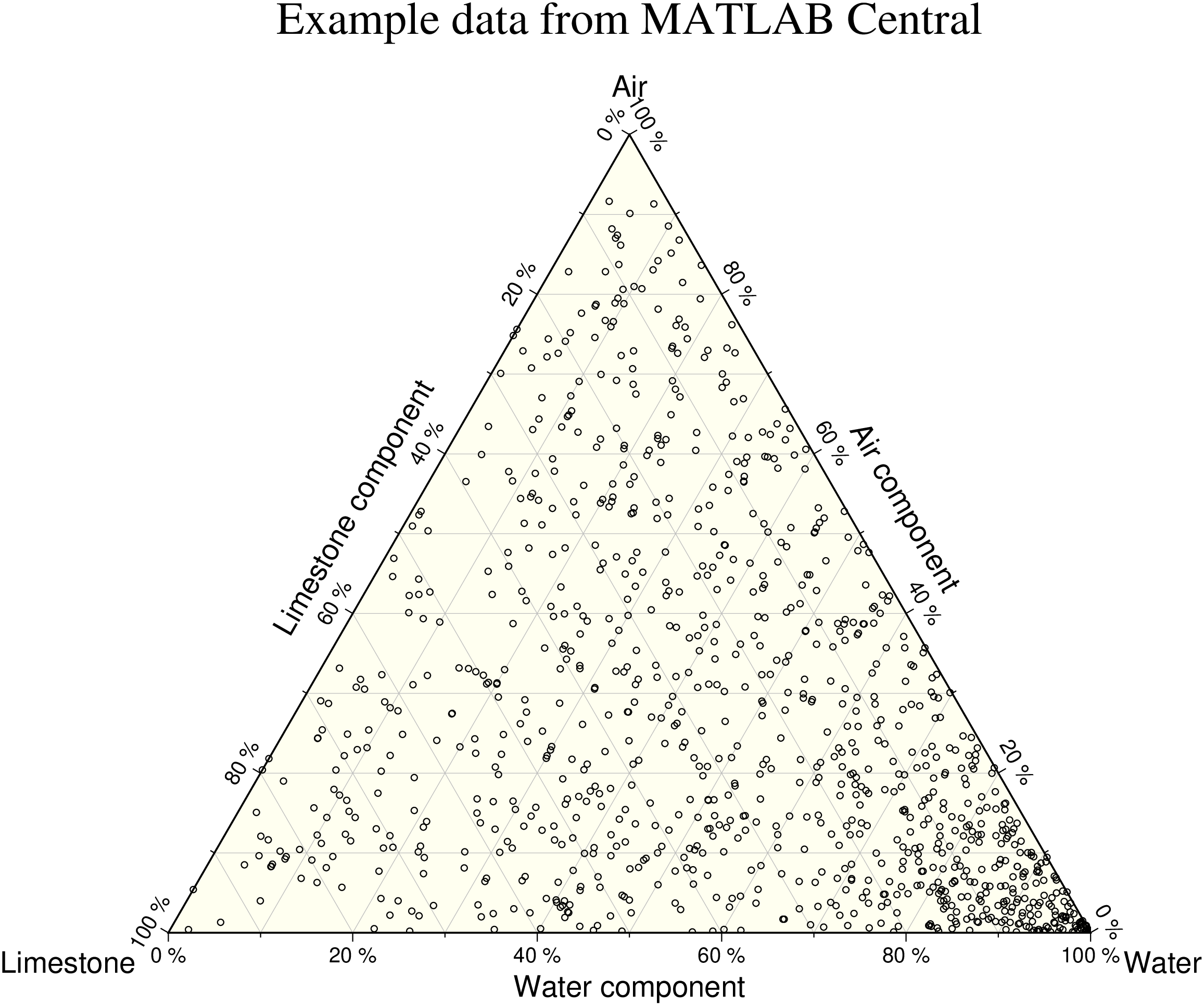
To plot circles (diameter = 0.1 cm) on a 6-inch-wide ternary diagram at the positions listed in the file ternary.txt, with default annotations and gridline spacings, using the specified labeling, try

using GMT

makecpt(cmap=:turbo, range=(0,80,10))
ternary("@ternary.txt", region=(0,100,0,100,0,100), marker=:circ, ms=0.1, vertex_labels="Water/Air/Limestone",
    frame=(annot=:auto, grid=:a, ticks=:a, alabel="Water component", blabel="Air component", clabel="Limestone component", suffix=" %", fill=:ivory, title="Example data from MATLAB Central"), show=true)

See other examples at Ternary plots

See Also