Leland Brown's "texture shading"
This tutorial starts with the examples shown by @KristofKoch in the Github issue that lead to inclusion of Leland Brown's "texture shading" technique in the GMT lib (not in any executable sofar) and postior wrapping in Julia GMT.jl
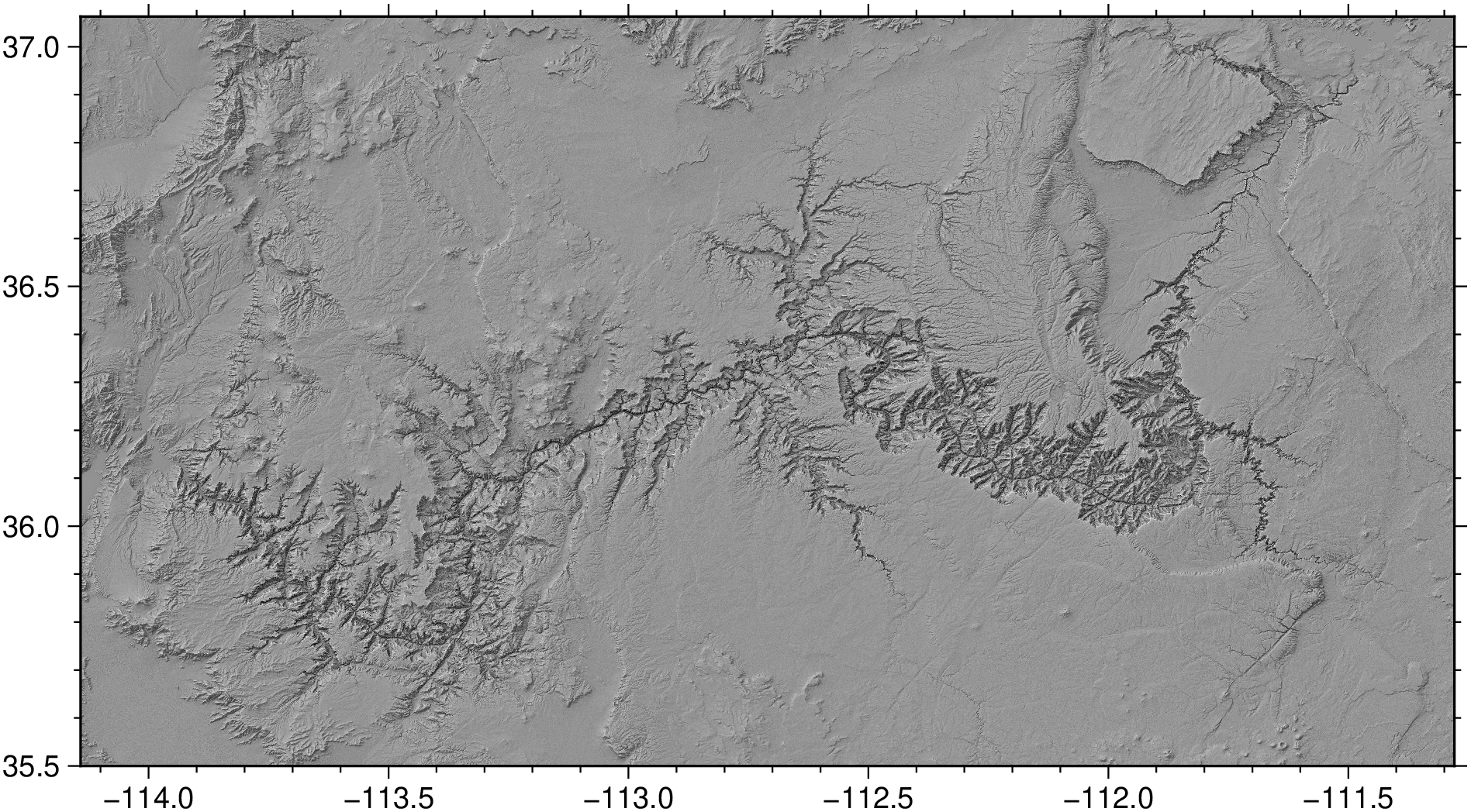
For the time being it is a set of examples on how to use the lelandshade and dependent functions. In the first example we get a demo grid from the GMT server and build a texture shaded image showing the inners of the calculation.
using GMT

# Extract a region from the SRTM1 grids stored in the GMT server
G = gmtread("@earth_relief_01s_g", region=(-114.14,-111.28,35.50,37.06));

# Compute the Leland texture
I1 = texture_img(G);

# Compute the grid's hillshade using GDAL's gdaldem program
Ihill = gdaldem(G, "hillshade", zfactor=3);     # The zfactor=3 is a terrain amplification factor

# Blend both images and Viz it.
I2 = blendimg!(I1, Ihill, new=true, transparency=0.6);
viz(I2)
The new=true option above forced the creation of the new array I2, but we could have just done blendimg!(I1, Ihill, transparency=0.6) and the final image would be stored in (overritten) I1. That is what is implemented in the wrapper function lelandshade that aglutinates all of the above steps, plus some extra options, in a single function.
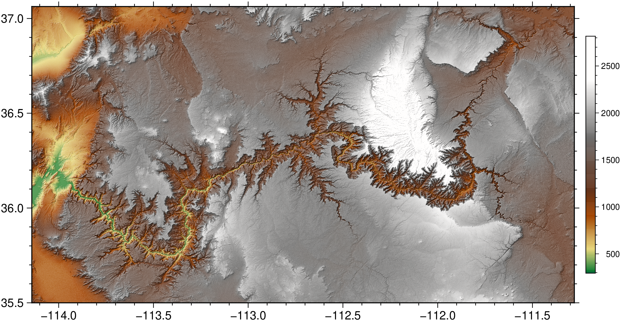
Map again the same refion but using this time a linear color scale. Since the G grid object is originated from the SRTM1 (1 arc second = ~30 m) stored in the GMT store, it comes with the indication of a default color map (geo) and is what we see (but we can select any cmap that we want).
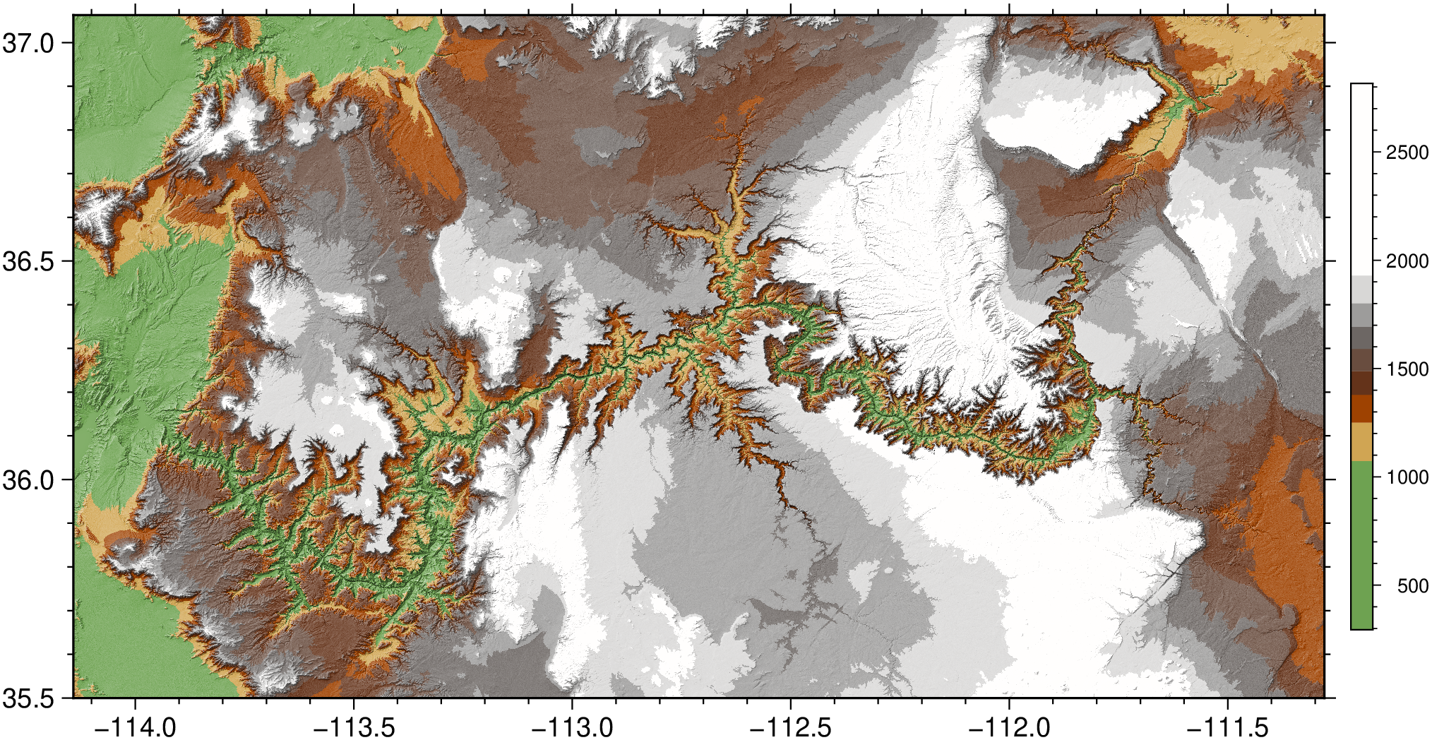
lelandshade(G, color=true, colorbar=true, show=true)A variation of the above is to make the color image with equalized color distribution where each color covers approximatelly the same area in the figure. We do that using the equalize=true option.
lelandshade(G, color=true, equalize=true, colorbar=true, show=true)The effect of the transparency option.
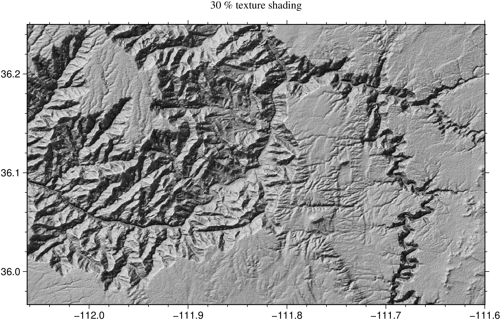
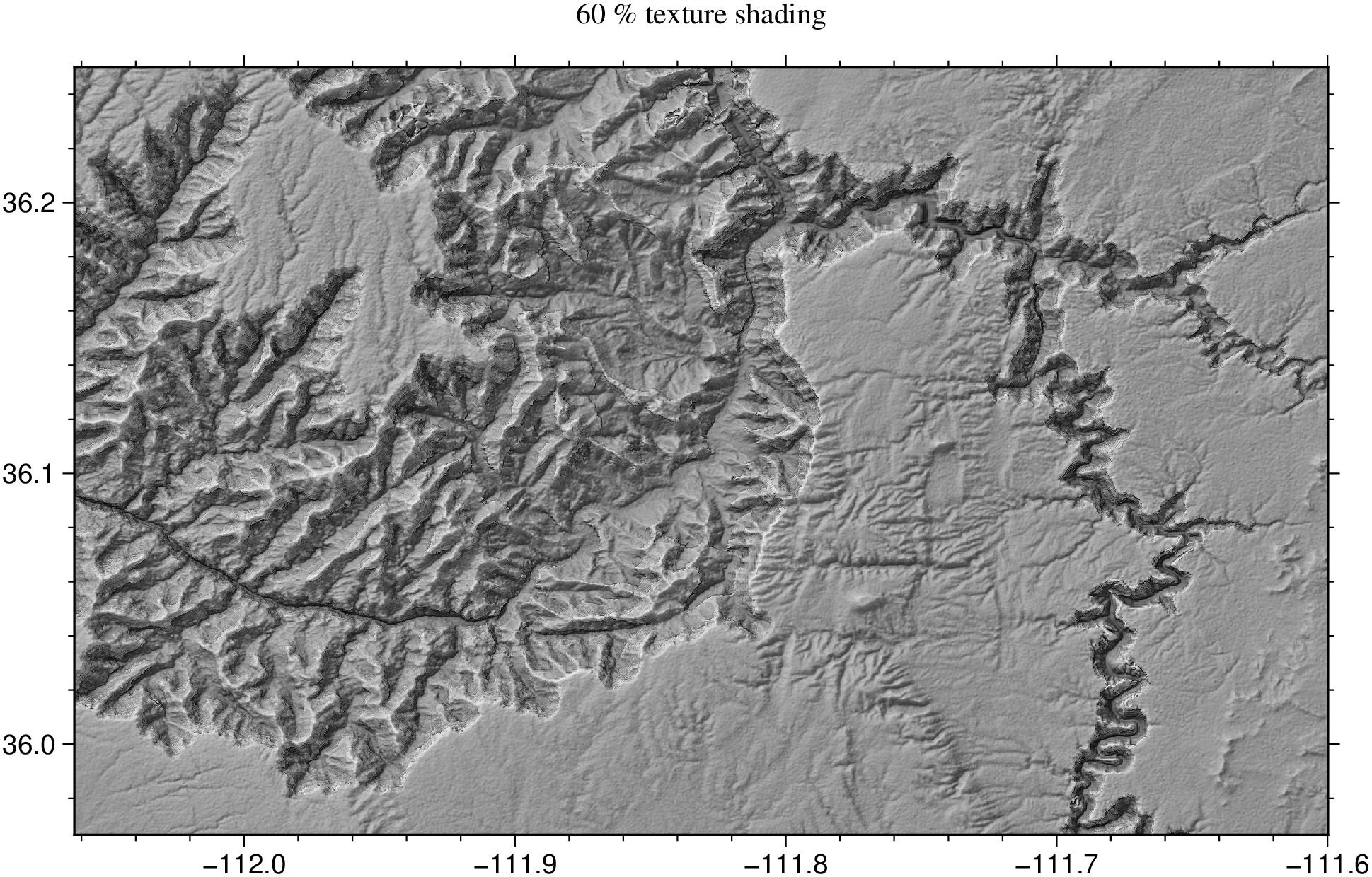
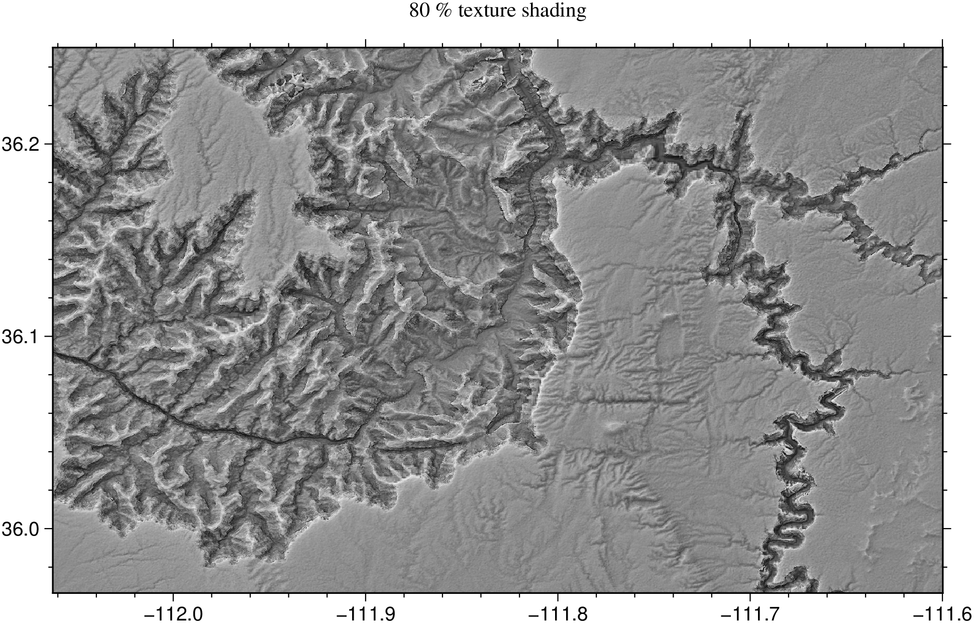
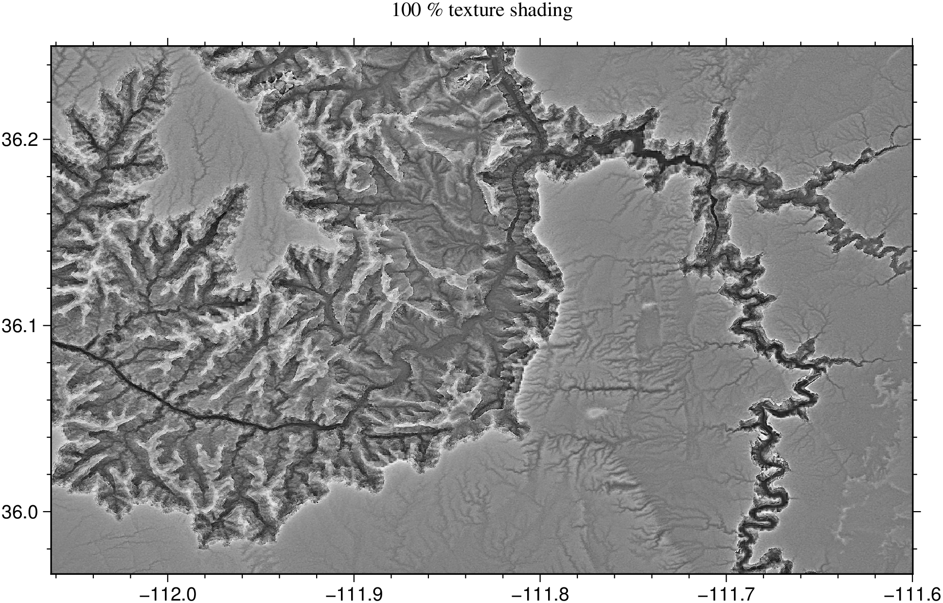
The examples shown above all used a transparency=0.6. Remember (from the manual) that the transparency represent the weight of the img2 with respect to img1 in the blend img1 + img2. So, when we used transparency=0.6 explicitly in the first example, or implicitly in the 2nd and 3rth examples, we imposed that the texture image weighted 60% and the hillshade 40%. This parameter has a relevant importance in the final image, so let us see examples of it by varying the amount of transparency in the mixture. And for better appreciate it we will use grayscale images and over a smaller region.
G = gmtread("@earth_relief_01s_g", region=(-112.06, -111.60, 35.97, 36.25));
lelandshade(G, transparency=0.0, title="0 % texture shading", par=(FONT_TITLE=10,), show=true)
lelandshade(G, transparency=0.3, title="30 % texture shading", par=(FONT_TITLE=10,), show=true)lelandshade(G, transparency=0.6, title="60 % texture shading", par=(FONT_TITLE=10,), show=true)lelandshade(G, transparency=0.8, title="80 % texture shading", par=(FONT_TITLE=10,), show=true)lelandshade(G, transparency=1.0, title="100 % texture shading", par=(FONT_TITLE=10,), show=true)Other than the transparency, several other parameters influence the look of the texture shaded images. Consult the lelandshade manual to learn about them.
These docs were autogenerated using GMT: v1.16.0
