using GMT

x = 1:50;
y = -0.3*x + 2*randn(50);
p = polyfit(x,y,1);

f = polyval(p,x);       # Evaluate the fitted polynomial p at the points in x.
plot(x,y,marker=:circ, legend="data")
plot!(x, f, lc=:brown, legend="linear fit", show=true)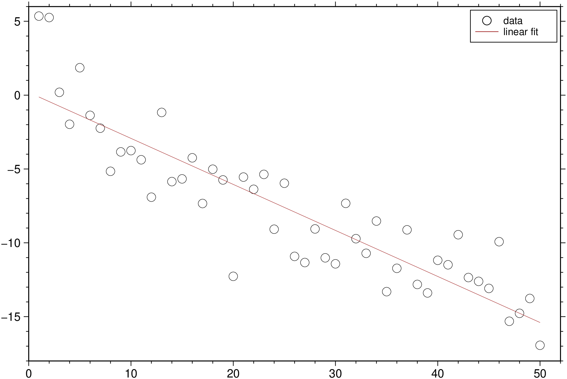
p = polyfit(x, y, n=length(x)-1; xscale=1)Returns the coefficients for a polynomial p(x) of degree n that is the least-squares best fit for the data in y. The coefficients in p are in ascending powers, and the length of p is n+1, where
\[p(x) = p[1] + p[2]x + p[3]x^2 + \ldots + p[n+1]x^n\]
The xscale parameter is useful when needing to get coeficients in different x units. For example when converting months or seconds into years.
Fit a simple linear regression model to a set of discrete 2-D data points.
Create a few vectors of sample data points (x,y). Fit a first degree polynomial to the data.
using GMT
x = 1:50;
y = -0.3*x + 2*randn(50);
p = polyfit(x,y,1);
f = polyval(p,x); # Evaluate the fitted polynomial p at the points in x.
plot(x,y,marker=:circ, legend="data")
plot!(x, f, lc=:brown, legend="linear fit", show=true)
This function has multiple methods:
polyfit(x, y, n::Int64; xscale) - utils.jl:1059polyfit(D::GMTdataset, n::Int64; xscale) - utils.jl:1058polyfit(x, y; ...) - utils.jl:1059polyfit(D::GMTdataset; ...) - utils.jl:1058