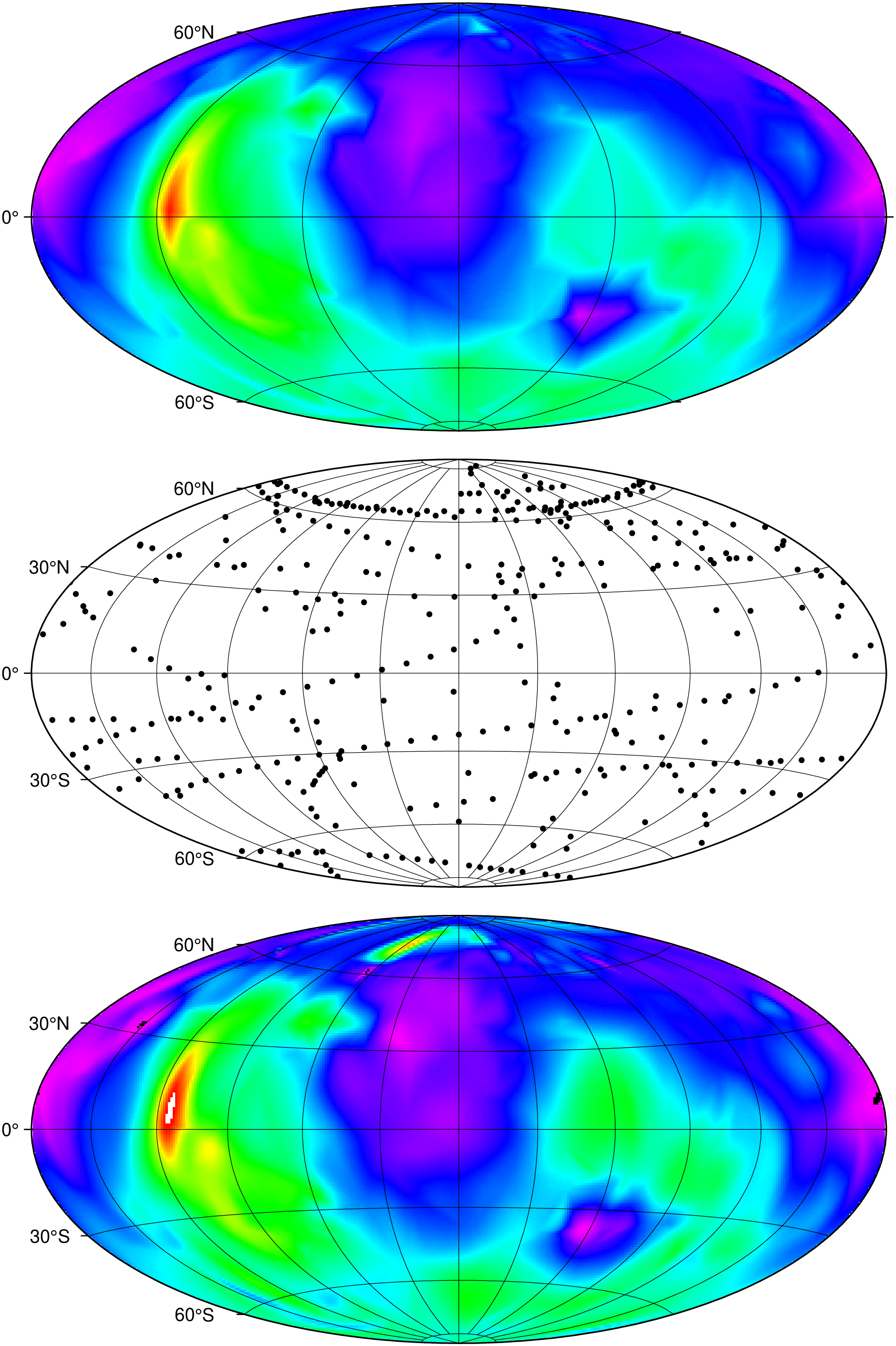
The next script produces the plot in Figure. Here we demonstrate how [sphinterpolate] can be used to perform spherical gridding. Our example uses early measurements of the radius of Mars from Mariner 9 and Viking Orbiter spacecrafts. The middle panels shows the data distribution while the top and bottom panel are images of the interpolation using a piecewise linear interpolation and a smoothed spline interpolation, respectively. For spherical gridding with large volumes of data we recommend [sphinterpolate] while for small data sets (such as this one, actually) you have more flexibility with [greenspline].
usingGMTresetGMT() # hide# Interpolate data of Mars radius from Mariner9 and Viking Orbiter spacecraftsmakecpt(cmap=:rainbow, range=(-7000,15000))# Piecewise linear interpolation; no tensionGtt =sphinterpolate("@mars370d.txt", region=:global, inc=1, tension=0)grdimage(Gtt, proj=:Hammer, figsize=15, frame=(annot=:auto, grid=:auto), yshift=18)plot!("@mars370d.txt", marker=:circle, ms=0.1, fill=0, frame=(annot=30, grid=30), yshift=-8)# SmoothingGtt =sphinterpolate("@mars370d.txt", region=:global, inc=1, tension=3)grdimage!(Gtt, frame=(annot=30, grid=30), yshift=-8, show=true)