using GMT

D = gmtread(TESTSDIR * "/assets/nmr_with_weights_and_x.csv");
D2 = whittaker(D, 2e4, 2);
D3 = whittaker(D, 2e4, 3);
plot(D)
plot!(D2, lc=:red, lt=1, legend="Degree 2")
plot!(D3, lc=:blue, lt=1, legend="Degree 3", show=true)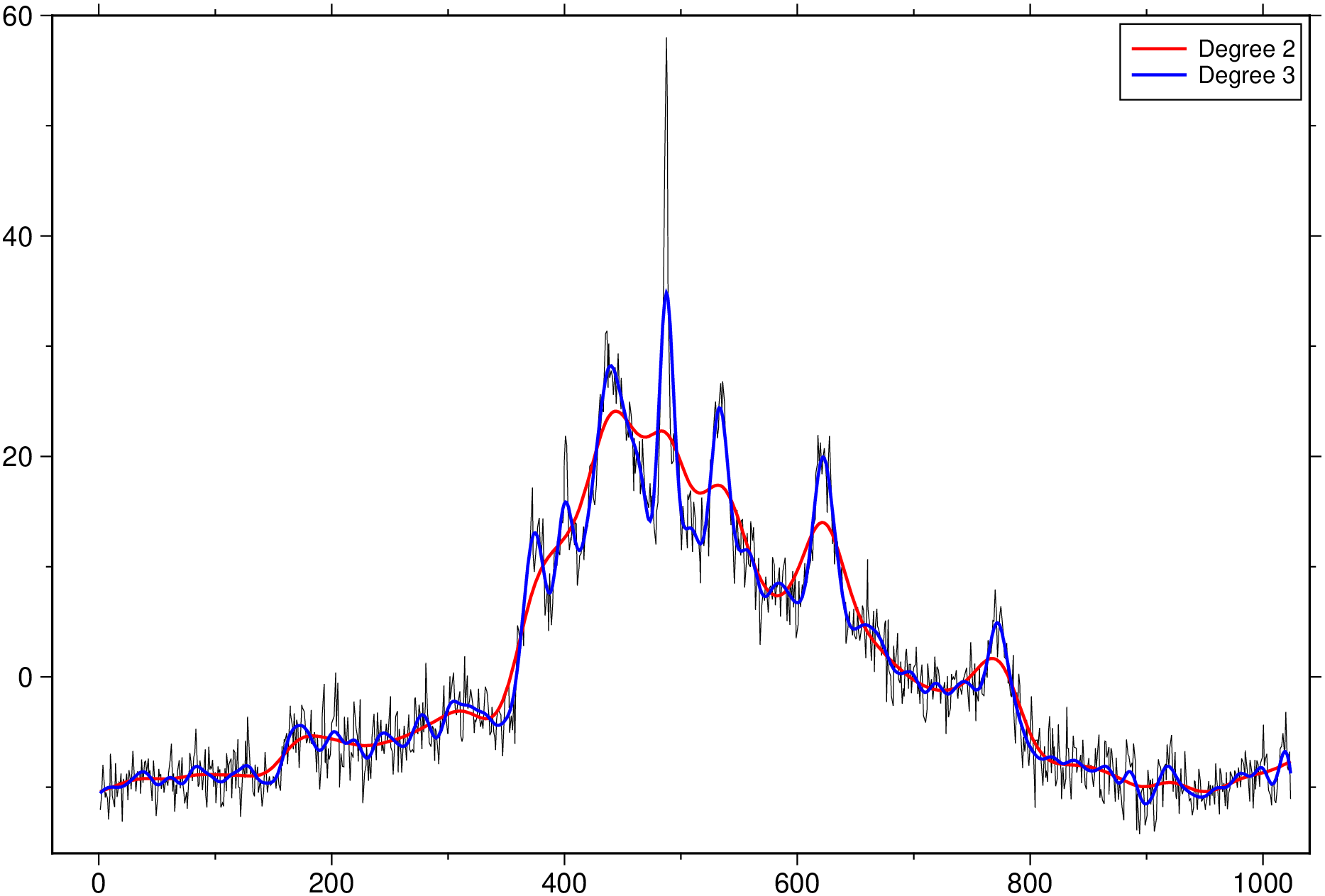
Dout = whittaker(D::GMTdataset, lambda, d=2; weights=nothing)or
z = whittaker(x::AbstractVecOrMat{<:Real}, y::VecOrMat{<:Real}, lambda, d=2; weights=nothing)Perform a Whittaker-Henderson smoothing and interpolation.
D: A GMTdatset with a x,y data series.x,y: In alternative to the D form, pass vectors of x and y.lambda: Smoothing parameter; large lambda gives smoother result.d: Order of differences (default = 2).weights: Weights (0/1 for missing/non-missing data). Note, if input y contains NaNs, we replace them by a another flag value and automatically set w.using GMT
D = gmtread(TESTSDIR * "/assets/nmr_with_weights_and_x.csv");
D2 = whittaker(D, 2e4, 2);
D3 = whittaker(D, 2e4, 3);
plot(D)
plot!(D2, lc=:red, lt=1, legend="Degree 2")
plot!(D3, lc=:blue, lt=1, legend="Degree 3", show=true)
t = 2001:0.003:2007;
_v = 5*cospi.((t .- 2000)/2); v = _v + (5*rand(length(t)) .- 2.5);
v[2002.6 .< t .< 2003.4] .= NaN;
z = whittaker(t, v, 0.01, 3);
plot(t, v, legend="Noisy", plot=(data=[t _v], lc=:green, lt=1, legend="Original"))
plot!(t, z, lc=:red, lt=1, legend="Degree 3", show=true)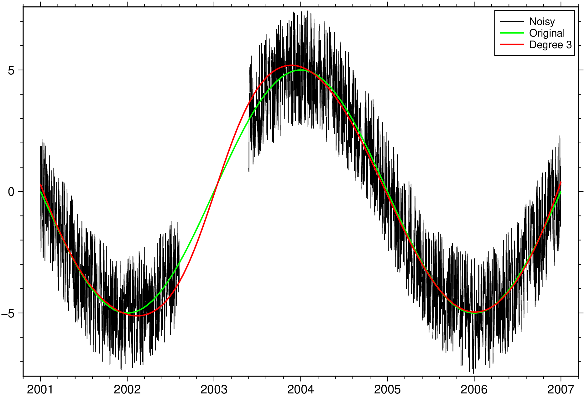
This function has multiple methods:
whittaker(x::AbstractVecOrMat{<:Real}, y::AbstractVecOrMat{<:Real}, lambda::Real; ...) - whittaker.jl:62whittaker(D::GMTdataset, lambda::Real, d::Int64; weights) - whittaker.jl:45whittaker(y::AbstractVecOrMat{<:Real}, lambda, d; weights, checkedNaN) - whittaker.jl:86whittaker(D::GMTdataset, lambda::Real; ...) - whittaker.jl:45whittaker(y::AbstractVecOrMat{<:Real}, lambda; ...) - whittaker.jl:86whittaker(x::AbstractVecOrMat{<:Real}, y::AbstractVecOrMat{<:Real}, lambda::Real, d::Int64; weights, checkedNaN) - whittaker.jl:62