symlog

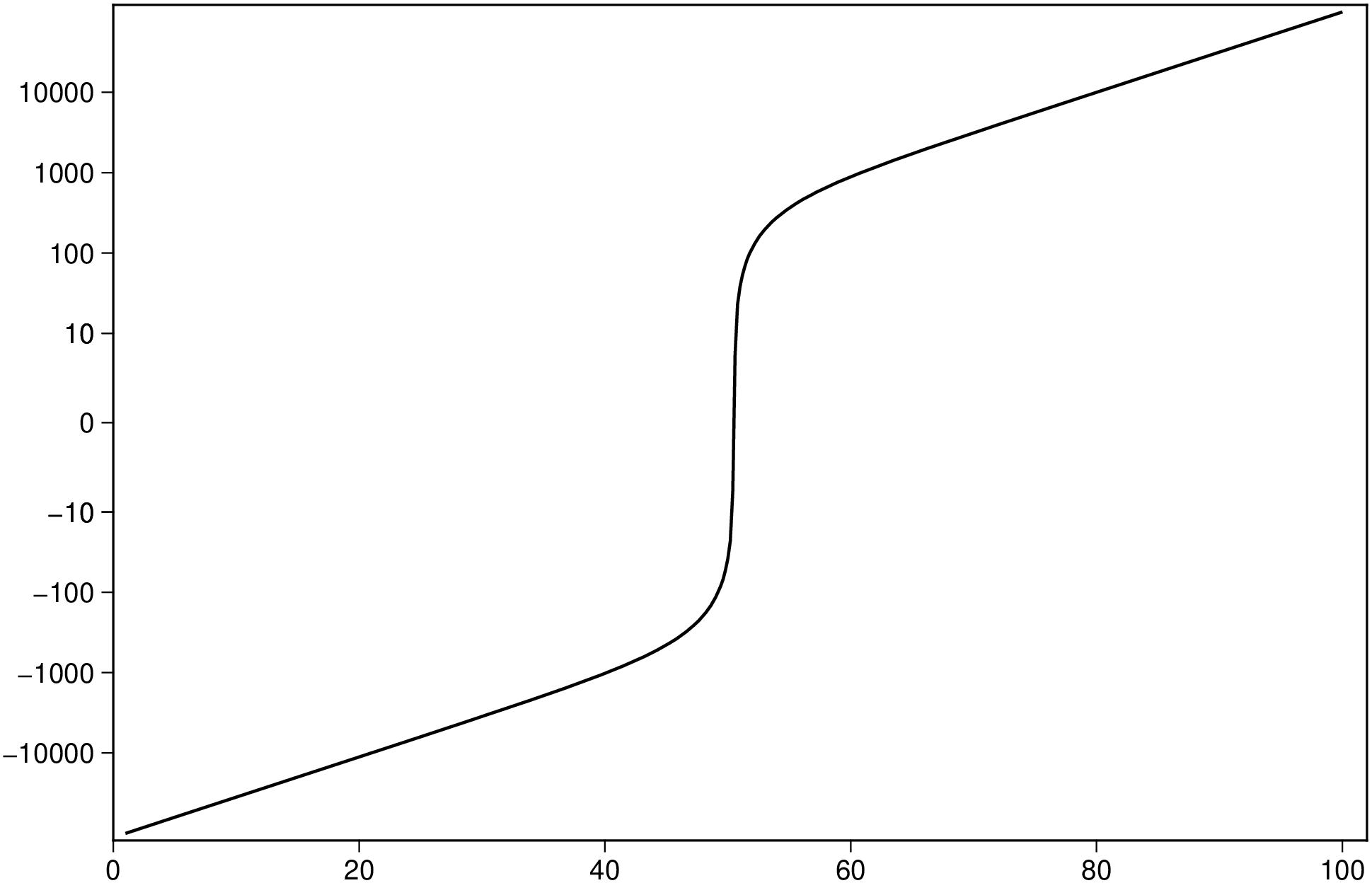
symlog(x, y; axis=:y, linthresh=1, linscale=1, base=10, kwargs...)

Plot data with a symmetric logarithmic scale, like matplotlib’s symlog. The scale is linear in the range [-linthresh, linthresh] and logarithmic beyond, allowing visualization of data that spans many orders of magnitude including negative values and zero.

symlog(x::AbstractVector, y::AbstractVector; axis=:y, linthresh=1, kwargs...)

Plots vectors x and y applying the symlog transform to the axis specified by axis.

symlog(D::GMTdataset; axis=:y, linthresh=1, kwargs...)

Plots a GMTdataset applying the symlog transform.

symlog(D::Vector{<:GMTdataset}; axis=:y, linthresh=1, kwargs...)

Plots multiple datasets, each with the symlog transform applied.

• axis: Which axis to transform. Use :y (default), :x, or :xy for both axes.
• linthresh: The range within which the plot is linear. This avoids having the plot go to infinity around zero (default: 1).
• linscale: This allows the linear range (-linthresh to linthresh) to be stretched relative to the logarithmic range. Its default value is 1.
• base: Base of the logarithm (default: 10).
• All other keyword arguments are forwarded to plot.

The inverse transform is available via isymlog(y; linthresh, linscale, base) to convert transformed values back to the original scale.

This module is a subset of plot. So not all (fine) controlling parameters are not listed here. For the finest control, user should consult the plot module.

Parameters

• B or axes or frame
  Set map boundary frame and axes attributes. Default is to draw and annotate left, bottom and vertical axes and just draw left and top axes. More at frame

• R or region or limits : – limits=(xmin, xmax, ymin, ymax) | limits=(BB=(xmin, xmax, ymin, ymax),) | limits=(LLUR=(xmin, xmax, ymin, ymax),units=“unit”) | …more
  Specify the region of interest. More at limits. For perspective view view, optionally add zmin,zmax. This option may be used to indicate the range used for the 3-D axes. You may ask for a larger w/e/s/n region to have more room between the image and the axes.

• U or time_stamp : – time_stamp=true | time_stamp=(just=“code”, pos=(dx,dy), label=“label”, com=true)
  Draw GMT time stamp logo on plot. More at timestamp

• V or verbose : – verbose=true | verbose=level
  Select verbosity level. More at verbose

• X or xshift or x_offset : xshift=true | xshift=x-shift | xshift=(shift=x-shift, mov=“a|c|f|r”)
  Shift plot origin. More at xshift

• Y or yshift or y_offset : yshift=true | yshift=y-shift | yshift=(shift=y-shift, mov=“a|c|f|r”)
  Shift plot origin. More at yshift

• figname or savefig or name : – figname=name.png
  Save the figure with the figname=name.ext where ext chooses the figure image format.

Examples

A curve spanning several orders of magnitude in both positive and negative directions. The symlog scale compresses the extremes while keeping a linear region near zero.

using GMT
x = collect(range(1.0, 100.0, length=500))
y = @. 10.0^(x/20) - 10.0^((101-x)/20)
symlog(x, y, linthresh=10, lw=1, show=true)

Apply the symlog transform to the X axis instead of Y.

using GMT
x = collect(range(1.0, 100.0, length=500))
y = @. 10.0^(x/20) - 10.0^((101-x)/20)
symlog(y, x, axis=:x, linthresh=10, lw=1, show=true)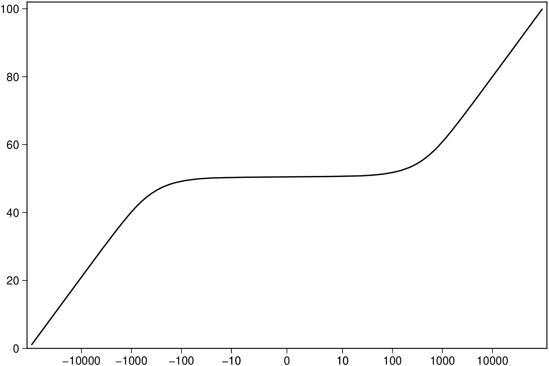

Apply the symlog transform to both axes.

using GMT
x = collect(range(-500.0, 500.0, length=1000))
y = @. x^3 / 1000
symlog(x, y, axis=:xy, linthresh=5, lw=1, show=true)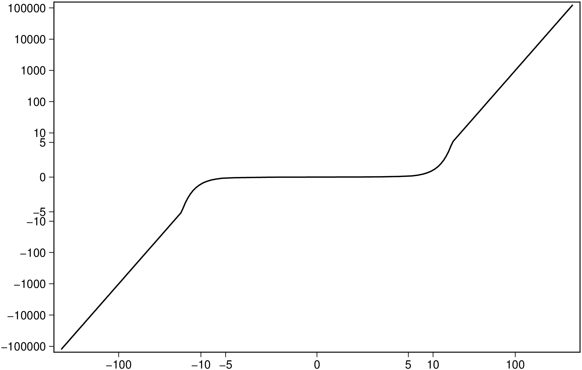

Source Code

This function has multiple methods:

• symlog(D::Vector{<:GMTdataset}; axis, linthresh, linscale, base, first, kwargs...) - symlog.jl:37
• symlog(D::GMTdataset; axis, linthresh, linscale, base, first, kwargs...) - symlog.jl:30
• symlog(x::AbstractVector{<:Real}, y::AbstractVector{<:Real}; axis, linthresh, linscale, base, first, kwargs...) - symlog.jl:23