using GMT

# Create focal mechanism data
D = mat2ds([0.0 5.0 0.0 0 90 0 5 0 0], ["Right Strike Slip"])

# Plot with fixed size beachballs
meca(D, region=(-1,4,1,6), proj=:Mercator, aki=2.5, fill=:black, show=true)
meca(cmd0::String="", arg1=nothing; kwargs...)meca - Plot focal mechanisms
Reads data values from tables or input arguments and plots focal mechanisms (beachballs). The module reads focal mechanism parameters and plots the corresponding beachballs on a map. Several input format conventions are supported: Aki & Richards, Global CMT, moment tensor, partial focal mechanism, and principal axis.
Columns: lon, lat, depth, strike, dip, rake, magnitude, newlon, newlat, text
Columns: lon, lat, depth, strike1, dip1, rake1, strike2, dip2, rake2, mantissa, exponent, newlon, newlat, text
Columns: lon, lat, depth, mrr, mtt, mff, mrt, mrf, mtf, exponent, newlon, newlat, text
Columns: lon, lat, depth, strike1, dip1, strike2, fault_type, magnitude, newlon, newlat, text
Columns: lon, lat, depth, T_value, T_azim, T_plunge, N_value, N_azim, N_plunge, P_value, P_azim, P_plunge, exponent, newlon, newlat, text
table
A data table (or matrices/datasets) containing focal mechanism parameters. The format depends on the convention specified.
J or proj or projection : – proj=
Select map projection. More at proj
R or region or limits : – limits=(xmin, xmax, ymin, ymax) | limits=(BB=(xmin, xmax, ymin, ymax),) | limits=(LLUR=(xmin, xmax, ymin, ymax),units=“unit”) | …more
Specify the region of interest. More at limits. For perspective view view, optionally add zmin,zmax. This option may be used to indicate the range used for the 3-D axes. You may ask for a larger w/e/s/n region to have more room between the image and the axes.
S or convention : Convention-specific options
Selects the input convention and symbol size. Choose from:
Append scale to set the symbol size. Use tuple form to add modifiers:
aki=(scale=val, ...) or CMT=(scale=val, ...) etc.Available modifiers (as named tuple elements):
A or offset : – offset=true | offset=(fill=…, offset=.., pen=…, size=…)
Offsets beachballs to the longitude, latitude specified in the last two columns of the input. A line connects the original and relocated positions. Available modifiers:
B or axes or frame
Set map boundary frame and axes attributes. Default is to draw and annotate left, bottom and vertical axes and just draw left and top axes. More at frame
C or color or cmap : – cmap=cpt
Give a CPT to determine compressive quadrant fill based on depth (3rd column).
D or depth_range : – depth_range=(depmin,depmax)
Plot only events with depths between depmin and depmax.
E or extensionfill : – extensionfill=fill
Selects filling of extensive quadrants [Default is white].
F : – Fa=true | Fa=[size[/Psymbol[Tsymbol]]] , Fe|Fg|Fr=fill , Fp|Ft|Fz=pen , Fo=true
Aliases:
G or fill or extensionfill : – fill=color
Selects filling of compressive quadrants [Default is black].
H or scale : – scale=true | scale=scale
Scale symbol sizes and pen widths on a per-record basis using the scale read from the data file. The symbol size is either provided by convention or via the input size column. Alternatively, append a constant scale that should be used instead of reading a scale column.
I or intens or intensity : – intens=val | intens=:a
Use the supplied intens value (nominally in the ±1 range) to modulate the compressional fill color by simulating illumination [none]. If no intensity is provided we will instead read intens from an extra data column after the required input columns determined by convention.
L or pen_outline : – pen_outline=pen
Draws the “beach ball” outline using specified pen attributes.
M or same_size or samesize : – same_size=true
Use the same size for all beachballs. Size is set from the magnitude columns, but the same size is used regardless of magnitude.
N or no_clip or noclip : – no_clip=true
Do NOT skip symbols that fall outside the map border [Default clips symbols].
T or nodal : – nodal=plane | nodal=(plane=val, pen=…)
Plot nodal planes and circumference only. Specify which plane(s) to draw:
Use tuple form to set pen: nodal=(plane=0, pen=pen_spec)
For double couple mechanisms, the nodal option renders the beach ball transparent by drawing only the nodal planes and the circumference. For non-double couple mechanisms, nodal=0 option overlays best double couple transparently.
U or time_stamp : – time_stamp=true | time_stamp=(just=“code”, pos=(dx,dy), label=“label”, com=true)
Draw GMT time stamp logo on plot. More at timestamp
V or verbose : – verbose=true | verbose=level
Select verbosity level. More at verbose
W or pen : – pen=pen
Set pen attributes for features [Default pen is 0.25p,black,solid]. This setting applies to A, L, T, Fp, Ft, and Fz, unless overruled by options to those arguments. See also [Pen attributes]
X or xshift or x_offset : xshift=true | xshift=x-shift | xshift=(shift=x-shift, mov=“a|c|f|r”)
Shift plot origin. More at xshift
Y or yshift or y_offset : yshift=true | yshift=y-shift | yshift=(shift=y-shift, mov=“a|c|f|r”)
Shift plot origin. More at yshift
di or nodata_in : – nodata_in=??
Substitute specific values with NaN. More at
e or pattern : – pattern=??
Only accept ASCII data records that contain the specified pattern. More at
h or header : – header=??
Specify that input and/or output file(s) have n header records. More at
i or incol or incols : – incol=col_num | incol=“opts”
Select input columns and transformations (0 is first column, t is trailing text, append word to read one word only). More at incol
p or view or perspective : – view=(azim, elev)
Default is viewpoint from an azimuth of 200 and elevation of 30 degrees.
Specify the viewpoint in terms of azimuth and elevation. The azimuth is the horizontal rotation about the z-axis as measured in degrees from the positive y-axis. That is, from North. This option is not yet fully expanded. Current alternatives are:
bar3!) More at perspectiveq or inrows : – inrows=??
Select specific data rows to be read and/or written. More at
t or transparency or alpha: – alpha=50
Set PDF transparency level for an overlay, in (0-100] percent range. [Default is 0, i.e., opaque]. Works only for the PDF and PNG formats.
yx : – yx=true
Swap 1st and 2nd column on input and/or output. More at
Plot focal mechanisms using Aki-Richards convention:
using GMT
# Create focal mechanism data
D = mat2ds([0.0 5.0 0.0 0 90 0 5 0 0], ["Right Strike Slip"])
# Plot with fixed size beachballs
meca(D, region=(-1,4,1,6), proj=:Mercator, aki=2.5, fill=:black, show=true)
Plot using Global CMT convention with depth-based coloring:
# Background map
grdimage("@earth_relief", region=[-74,-59,5,15], proj=:guess, figsize=10, shade=true)
coast!(shorelines=true, borders=((type=1, pen=0.8),(type=2, pen=0.1)))

# Focal mechanisms with offsets
meca!("focal_data.txt", CMT=(scale=0.4, font=6), offset=true, fill=:black, show=true)
Plot multiple mechanisms with varying types:
using GMT

# Right lateral strike slip
D1 = mat2ds([0.0 5.0 0.0 0 90 0 5 0 0], ["Right Strike Slip"])
meca(D1, region=(-1,4,1,6), proj=:Mercator, aki=2.5, fill=:black)

# Thrust fault
D2 = mat2ds([0.0 3.5 0.0 0 45 90 5 0 0], ["Thrust"])
meca!(D2, aki=2.5, fill=:black)

# Normal fault
D3 = mat2ds([0.0 2.0 0.0 0 45 -90 5 0 0], ["Normal"])
meca!(D3, aki=2.5, fill=:black, show=true)
using GMT

psmeca([0.0 3.0 0.0 0 45 90 5 0 0], aki=true, fill=:black, region=(-1,4,0,6), proj=:Merc, show=1)
The same but add a Label
psmeca(mat2ds([0.0 3.0 0.0 0 45 90 5 0 0], ["Thrust"]), aki=true, fill=:black, region=(-1,4,0,6), proj=:Merc, show=1)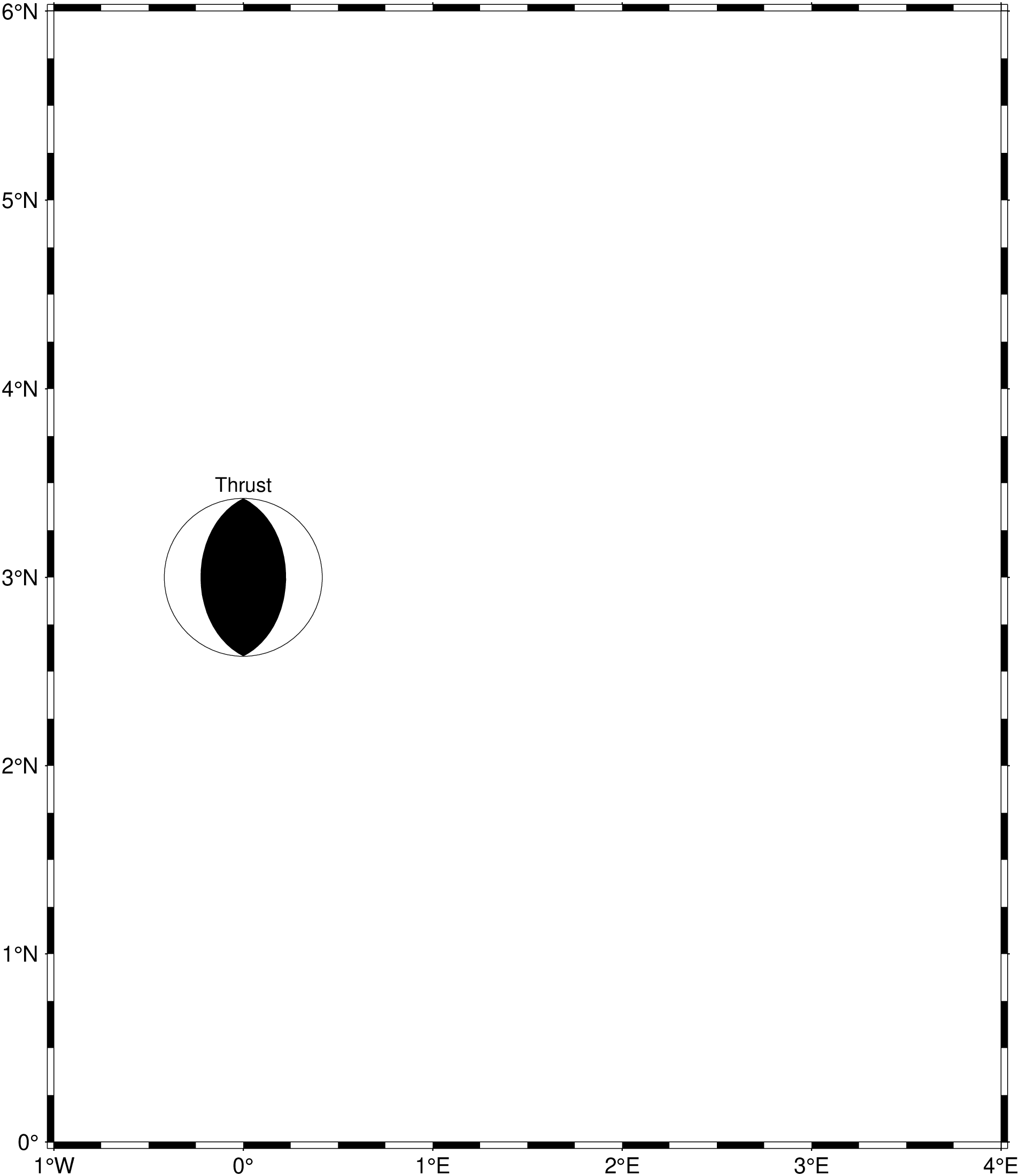
Aki, K., & Richards, P. G. (1980). Quantitative seismology: theory and methods. San Francisco: W. H. Freeman.
Dahlen, F. A., & Tromp, J. (1998). Theoretical global seismology. Princeton, N.J: Princeton University Press.
Frohlich, C. (1996). Cliff’s Nodes Concerning Plotting Nodal Lines for P, SH and SV. Seismological Research Letters, 67(1), 16–24, https://doi.org/10.1785/gssrl.67.1.16.
Lay, T., & Wallace, T. C. (1995). Modern global seismology. San Diego: Academic Press.
This function has multiple methods:
meca(cmd0::String; kwargs...) - psmeca.jl:77meca(arg1; kwargs...) - psmeca.jl:78