gmtbinstats

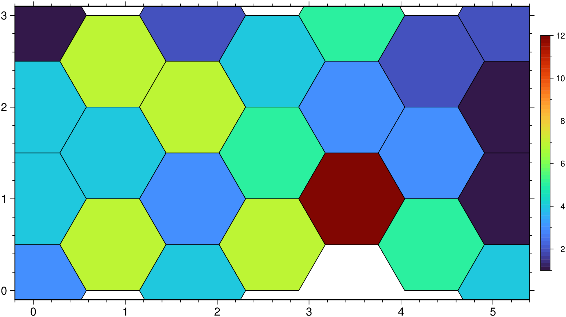
gmtbinstats(cmd0::String="", arg1=nothing; kwargs...)

Bin spatial data and determine statistics per bin.

Description

Reads arbitrarily located (x,y[,z][,w]) points (2-4 columns) and for each node in the specified grid layout determines which points are within the given radius. These point are then used in the calculation of the specified statistic. The results may be presented as is or may be normalized by the circle area to perhaps give density estimates. Alternatively, select hexagonal tiling instead or a rectangular grid layout.

Required Arguments

• table : – Either as a string with the filename in arg cmd0 or as Matrix or GMTdataset in arg1
  A 2-4 column matrix holding (x,y[,z][,w]) data values. You must use weights to indicate that you have weights. Only -Cn will accept 2 columns only.

• I or inc or increment or spacing : – inc=x_inc | inc=(x_inc, y_inc) | inc=“xinc[+e|n][/yinc[+e|n]]”
  Specify the grid increments or the block sizes. More at [spacing](../common_opts/opt_I.html)

• R or region or limits : – limits=(xmin, xmax, ymin, ymax) | limits=(BB=(xmin, xmax, ymin, ymax),) | limits=(LLUR=(xmin, xmax, ymin, ymax),units=“unit”) | …more
  Specify the region of interest. More at [limits](../common_opts/opt_R.html). For perspective view view, optionally add zmin,zmax. This option may be used to indicate the range used for the 3-D axes. You may ask for a larger w/e/s/n region to have more room between the image and the axes.

Optional Arguments

• C or stats or statistic : – stats=…
  Choose the statistic that will be computed per node based on the points that are within radius distance of the node. Select one of:

  • average or mean # mean (average)
  • mad # median absolute deviation
  • range # full (max-min) range
  • iq or interquartil # 25-75% interquartile range
  • min or minimum # minimum (low)
  • min_pos or minimum_pos # minimum of positive values only
  • median # median
  • number or count # number of values
  • LMS # LMS scale
  • mode # mode (maximum likelihood)
  • quantil[val] # selected quantile (append desired quantile in 0-100% range [50], e.g. “quantil25”)
  • rms # the r.m.s.
  • std # standard deviation
  • max or maximum # maximum (upper)
  • max_neg or maximum_neg # maximum of negative values only
  • sum # the sum

• nbins : – nbins=n
  Set the number of hexagonal cells along the horizontal direction. Grid increment (inc) is computed x-data range and this number of cells. Default, when figure size is known, uses a simple heuristic to st increment.

• threshold : – threshold=xx
  Rows with computed stats lower then threshold are removed. Note that this option is not to be used when computing grids (will be ignored).

• E or empty : – empty=-9999 Set the value assigned to empty nodes. By default we use NaN.

• N or normalize : – normalize=true
  Normalize the resulting grid values by the area represented by the search_radius [no normalization].

• S or search_radius : – search_radius=rad
  Sets the search radius that determines which data points are considered close to a node. Append the distance unit if wished. Not compatible with tiling.

• T or tiling or bins : – tiling=rectangular or tiling=hexagonal
  Instead of circular, possibly overlapping areas, select non-overlapping tiling. Choose between tiling=rectangular or tiling=hexagonal binning. For rectangular, set bin sizes via spacing and we write the computed statistics to the grid file. For tiling=hexagonal, we write a table with the centers of the hexagons and the computed statistics. Here, the spacing setting is expected to set the y increment only and we compute the x-increment given the geometry. Because the horizontal spacing between hexagon centers in x and y have a ratio of sqrt(3), we will automatically adjust xmax in region to fit a whole number of hexagons. Note: Hexagonal tiling requires Cartesian data.

• W or weights : – weights=true or weights=“+s”
  Input data have an extra column containing observation point weight. If weights are given then weighted statistical quantities will be computed while the count will be the sum of the weights instead of number of points. If your weights are actually uncertainties (one sigma) then use weights="+s" and we compute weight = 1/sigma.

• U or time_stamp : – time_stamp=true | time_stamp=(just=“code”, pos=(dx,dy), label=“label”, com=true)
  Draw GMT time stamp logo on plot. More at [timestamp](../common_opts/opt_U.html)

• V or verbose : – verbose=true | verbose=level
  Select verbosity level. More at [verbose](../common_opts/opt_V.html)

• a or aspatial : – aspatial=??
  Control how aspatial data are handled in GMT during input and output. More at

• bi or binary_in : – binary_in=??
  Select native binary format for primary table input. More at

• di or nodata_in : – nodata_in=??
  Substitute specific values with NaN. More at

• e or pattern : – pattern=??
  Only accept ASCII data records that contain the specified pattern. More at

• f or colinfo : – colinfo=??
  Specify the data types of input and/or output columns (time or geographical data). More at

• g or gap : – gap=??
  Examine the spacing between consecutive data points in order to impose breaks in the line. More at

• h or header : – header=??
  Specify that input and/or output file(s) have n header records. More at

• i or incol or incols : – incol=col_num | incol=“opts”
  Select input columns and transformations (0 is first column, t is trailing text, append word to read one word only). More at incol

• q or inrows : – inrows=??
  Select specific data rows to be read and/or written. More at

• r or reg or registration : – reg=:p | reg=:g
  Select gridline or pixel node registration. Used only when output is a grid. More at

• w or wrap or cyclic : – wrap=??
  Convert input records to a cyclical coordinate. More at

• yx : – yx=true
  Swap 1st and 2nd column on input and/or output. More at

Examples

To examine the population inside a circle of 1000 km radius for all nodes in a 5x5 arc degree grid, using the remote file @capitals.gmt, and plot the resulting grid using default projection and colors, try

G = gmtbinstats("@capitals.gmt", a="2=population", region=:global360, inc=5, stats=:sum, search_radius="1000k");
imshow(G)

Make a hexbin plot with random numbers.

xy = rand(100,2) .* [5 3];
D = binstats(xy, region=(0,5,0,3), inc=1, tiling=:hex, stats=:number);
imshow(D, hexbin=true, ml=0.5, colorbar=true)