using GMT
boxplot(randn(100,5), outliers=(size="5p",), ticks=["A","B","C","D","E"], fill=true, notch=true, show=true)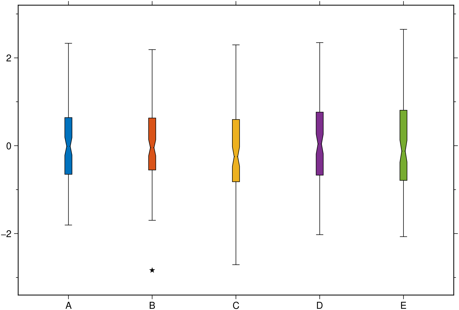
boxplot(data, grp=[]; pos=nothing, kwargs...)Draw a box-and-whisker style plot. The input data can take several different forms.
boxplot(data::AbstractVector{<:Real}; kwargs...)
Draws a single boxplot. Options in kwargs provide fine settings for the boxplot
boxwidth or cap: Sets the the boxplot width and, optionally, the cap width. Provide info as boxwidth="10p/3p" to set the boxwidth different from the cap’s. Note, however, that this requires GMT6.5. Previous versions do not destinguish box and cap widths.notch: Logical value indicating whether the box should have a notch (needs GMT6.5).outliers: If other than a NamedTuple, plots outliers (1.5IQR) with the default black 5pt stars. If argument is a NamedTuple (marker=??, size=??, color=??, markeredge=??), where marker is one of the plots marker symbols, plots the outliers with those specifications. Any missing spec default to the above values. i.e outliers=(size="3p") plots black 3 pt stars.fill: If fill=true paint the box with the first color of a pre-defined color scheme. Otherwise, give a color to paint the box.horizontal or hbar: Logical value indicating whether to plot horizontal instead of vertical boxplots.weights: Array giving the weights for the data in data. The array must be the same size as data.region or limits: By default we estimate the plotting limits but sometimes that may not be convenient. Give a region=(x_min,x_max,y_min,y_max) tuple if you want to control the plotting limits.ticks or xticks or yticks: A tuple with annotation location and label. E.g. xticks=([2], [“Ab”]) where first element is an AbstractArray and second an array or tuple of strings or symbols.boxplot(data::AbstractVector{<:Real}, grp::AbstractVector, ...) Use the categorical vector (made of integers or text strings) grp break down a the data column vector in cathegories (groups).
boxplot(data::AbstractMatrix{<:Real}; pos=Vector{<:Real}, ...) where pos is a coordinate vector (or a single location when data is a vector) where to plot the boxes. Default plots them at 1:n_boxes or 1:n_groups.
boxplot(data::GMTdatset{<:Real}; pos=Vector{Real}(), ...) Like the above case but the input data is stored in a GMTdataset
boxplot(data::Vector{Vector{<:Real}}; pos=Vector{Real}(), ...) Similar to the Matrix case but here each data vector used to compute the statistics can have a different number of points. There will be as many boxplots as length(data)
boxplot(data::Array{T<:Real,3}; pos=Vector{Real}(), groupwidth=0.75, ccolor=false, ...) Draws G groups of boxplots of N columns boxes. - groupWidth: Specify the proportion of the x-axis interval across which each x-group of boxes should be spread. The default is 0.75. - ccolor: Logical value indicating whether the groups have constant color (when fill=true is used) or have variable color (the default). - fill: If fill=true paint the boxes with a pre-defined color scheme. Otherwise, give a list of colors to paint the boxes. - fillalpha: When the fill option is used, we can set the transparency of filled violins with this option that takes in an array (vec or 1-row matrix) with numeric values between [0-1] or ]1-100], where 100 (or 1) means full transparency. - separator: If = true plot a black line separating the groups. Otherwise provide the pen settings of those lines. - ticks or xticks or yticks: A tuple with annotations interval and labels. E.g. xticks=(1:5, [“a”, “b”, “c”, “d”]) where first element is an AbstractArray and second an array or tuple of strings or symbols.
boxplot(data::Vector{Vector{Vector{<:Real}}}, ...) Like the above but here the groups (length(data)) can have a variable number of elements and each have its own size.
This module is a subset of plot. So not all (fine) controlling parameters are not listed here. For the finest control, user should consult the plot module. |
| Parameters |
B or axes or frame
Set map boundary frame and axes attributes. Default is to draw and annotate left, bottom and vertical axes and just draw left and top axes. More at frame
R or region or limits : – limits=(xmin, xmax, ymin, ymax) | limits=(BB=(xmin, xmax, ymin, ymax),) | limits=(LLUR=(xmin, xmax, ymin, ymax),units=“unit”) | …more
Specify the region of interest. More at limits. For perspective view view, optionally add zmin,zmax. This option may be used to indicate the range used for the 3-D axes. You may ask for a larger w/e/s/n region to have more room between the image and the axes.
U or time_stamp : – time_stamp=true | time_stamp=(just=“code”, pos=(dx,dy), label=“label”, com=true)
Draw GMT time stamp logo on plot. More at timestamp
V or verbose : – verbose=true | verbose=level
Select verbosity level. More at verbose
X or xshift or x_offset : xshift=true | xshift=x-shift | xshift=(shift=x-shift, mov=“a|c|f|r”)
Shift plot origin. More at xshift
Y or yshift or y_offset : yshift=true | yshift=y-shift | yshift=(shift=y-shift, mov=“a|c|f|r”)
Shift plot origin. More at yshift
figname or savefig or name : – figname=name.png
Save the figure with the figname=name.ext where ext chooses the figure image format.
Create a boxplot with five boxes, name each, plot the outliers, colorize with the default color schema and add notches (this needs GMT >= 6.5).
using GMT
boxplot(randn(100,5), outliers=(size="5p",), ticks=["A","B","C","D","E"], fill=true, notch=true, show=true)
An horizontal boxplot with default colors, displaying outliers as 6p black stars. Noches are also shown but this requires GMT6.5.
using GMT
boxplot(randn(50,6), notch=true, fill=true, outliers=(size="6p",), hbar=true, show=1)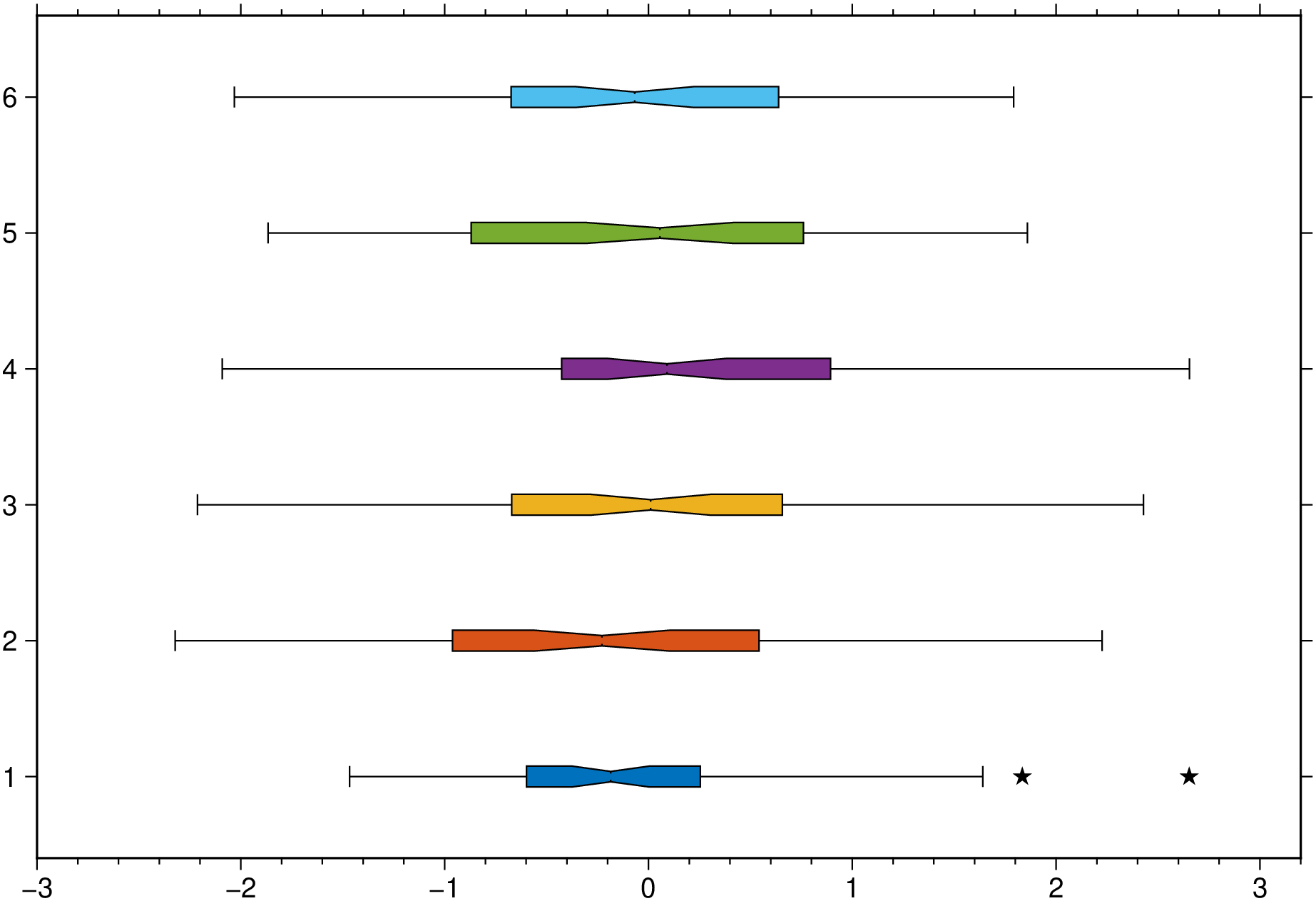
This function has multiple methods:
boxplot(data::Array{Array{Vector{T}, 1}, 1}; pos, first, groupwidth, ccolor, kwargs...) where T - statplots.jl:318boxplot(data::Array{T, 3}; pos, first, groupwidth, ccolor, kwargs...) where T - statplots.jl:279boxplot(data::GMTdataset; pos, first, kwargs...) - statplots.jl:248boxplot(data::Union{AbstractMatrix{T}, Array{Vector{T}, 1}}; pos, first, kwargs...) where T - statplots.jl:261boxplot(data::AbstractVector{<:Real}, grp::AbstractVector; pos, first, kwargs...) - statplots.jl:252boxplot(data::AbstractVector{<:Real}; ...) - statplots.jl:252