Tutorial 5 - 3-D Topography (Planetary / Antarctic maps) 🏔️#
In this tutorial, let’s use PyGMT to create 3-D perspective plots of Digital Elevation Models (DEM) over Mars (the planet) and Antarctica (the continent)!
Note
This tutorial is part of the AGU24 annual meeting GMT/PyGMT pre-conference workshop (PREWS9) Mastering Geospatial Visualizations with GMT/PyGMT
Website: https://www.generic-mapping-tools.org/agu24workshop
Conference: https://agu.confex.com/agu/agu24/meetingapp.cgi/Session/226736
History
Authors: Wei Ji Leong and André Belém
Created: November-December 2024
Recommended versions: PyGMT v0.13.0 with GMT 6.5.0
References
Fee free to play around with these code examples 🚀. In case you found any kind of error, just report it by opening an issue or provide a fix via a pull request. Please use the GMT forum to ask questions.
import pygmt
import rioxarray
import rioxarray.merge
0️⃣ Mars relief data#
First, we’ll load the Mars Orbiter Laser Altimeter (MOLA) dataset using
pygmt.datasets.load_mars_relief.
The following command will load the MOLA dataset into an
xarray.DataArray
grid, and we’ll set the resolution parameter to 01d (1 arc-degree) for now.
da_mars = pygmt.datasets.load_mars_relief(resolution="01d")
da_mars
gmtread [NOTICE]: Remote data courtesy of GMT data server oceania [http://oceania.generic-mapping-tools.org]
gmtread [NOTICE]: MOLA Mars Relief at 1x1 arc degrees reduced by Gaussian Cartesian filtering (167.7 km fullwidth) [Neumann et al., 2003].
gmtread [NOTICE]: -> Download grid file [109K]: mars_relief_01d_g.grd
<xarray.DataArray 'z' (lat: 181, lon: 361)> Size: 523kB
array([[ 3840.5,  3840.5,  3840.5, ...,  3840.5,  3840.5,  3840.5],
       [ 3712.5,  3697. ,  3674.5, ...,  3739. ,  3726. ,  3712.5],
       [ 2714.5,  2717. ,  2674.5, ...,  2917.5,  2808.5,  2714.5],
       ...,
       [-2523. , -2522. , -2533.5, ..., -2567.5, -2564. , -2523. ],
       [-2294. , -2300.5, -2303.5, ..., -2269.5, -2283.5, -2294. ],
       [-2019. , -2019. , -2019. , ..., -2019. , -2019. , -2019. ]])
Coordinates:
  * lat      (lat) float64 1kB -90.0 -89.0 -88.0 -87.0 ... 87.0 88.0 89.0 90.0
  * lon      (lon) float64 3kB -180.0 -179.0 -178.0 -177.0 ... 178.0 179.0 180.0
Attributes:
    Conventions:  CF-1.7
    title:        MOLA Mars Relief at 01 arc degree
    history:
    description:  NASA Mars (MOLA) relief
    long_name:    elevation (m)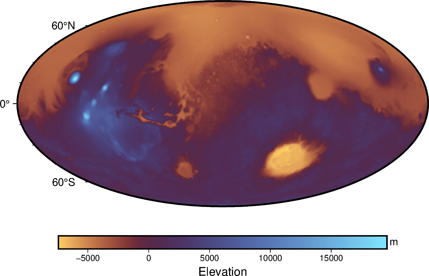
units: meters0.1 2-D map view#
Here we can create a map of the entire Martian surface, using a
Mollweide projection.
To get a reddish hue, we’ll use a
colormap
called SCM/managua which comes with a soft hinge
(see makecpt -C)
that can be set at elevation 0 meter by appending +h0 to the cmap parameter.
fig = pygmt.Figure()
fig.grdimage(grid=da_mars, frame=True, projection="W12c", cmap="SCM/managua+h0")
fig.colorbar(frame=["a5000", "x+lElevation", "y+lm"])
fig.show()
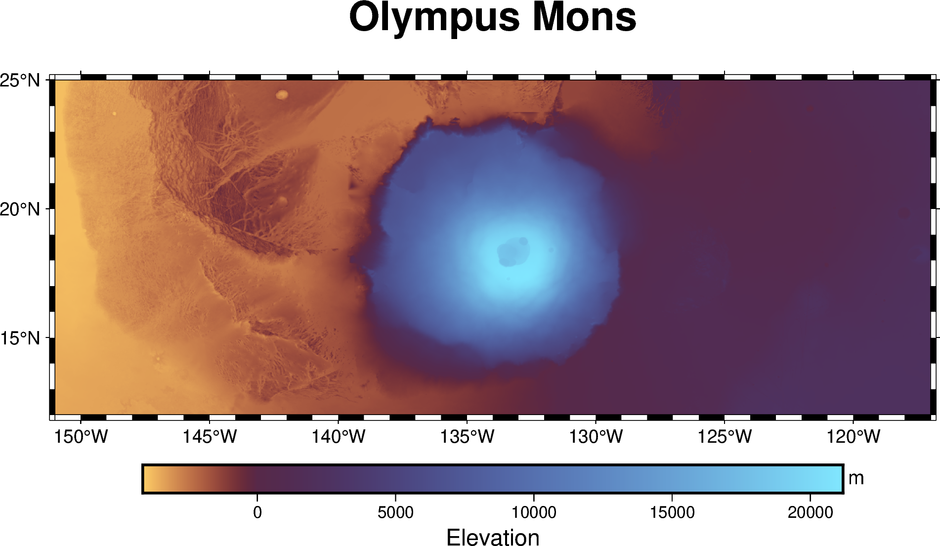
0.2 Zoomed in view#
A very interesting feature is Olympus Mons centered at approximately 19°N and 133°W, with a height of 22 km (14 miles) and approximately 700 km (435 miles) in diameter.
Let’s grab a higher resolution map over the volcano, and plot another 2-D map!
da_olympus = pygmt.datasets.load_mars_relief(
    resolution="30s",  # 30 arc-seconds
    region=[-151, -117, 12, 25],  # xmin, xmax, ymin, ymax
)
da_olympus
grdblend [NOTICE]: Remote data courtesy of GMT data server oceania [http://oceania.generic-mapping-tools.org]
grdblend [NOTICE]: MOLA Mars Relief at 30x30 arc seconds reduced by Gaussian Cartesian filtering (1.4 km fullwidth) [Neumann et al., 2003].
grdblend [NOTICE]: -> Download 15x15 degree grid tile (mars_relief_30s_g): N00W165
<xarray.DataArray 'z' (lat: 1561, lon: 4081)> Size: 51MB
array([[-3492. , -3491. , -3491. , ...,  2432. ,  2432.5,  2432.5],
       [-3492. , -3491. , -3491. , ...,  2432. ,  2431.5,  2432. ],
       [-3492. , -3491. , -3491. , ...,  2431.5,  2431. ,  2431. ],
       ...,
       [-3872. , -3872. , -3872. , ...,  1926.5,  1929.5,  1932.5],
       [-3872. , -3872. , -3872. , ...,  1925.5,  1928. ,  1931. ],
       [-3872. , -3872. , -3872. , ...,  1923.5,  1925.5,  1928. ]])
Coordinates:
  * lat      (lat) float64 12kB 12.0 12.01 12.02 12.03 ... 24.98 24.99 25.0
  * lon      (lon) float64 33kB -151.0 -151.0 -151.0 ... -117.0 -117.0 -117.0
Attributes:
    Conventions:  CF-1.7
    title:
    history:      gmt grdblend @mars_relief_30s_g/ -R-151/-117/12/25 -I30s -r...
    description:  NASA Mars (MOLA) relief
    long_name:    z
units: metersfig = pygmt.Figure()
fig.grdimage(grid=da_olympus, frame=["WSne+tOlympus Mons", "af"], cmap="SCM/managua+h0")
fig.colorbar(frame=["a5000", "x+lElevation", "y+lm"])
fig.show()
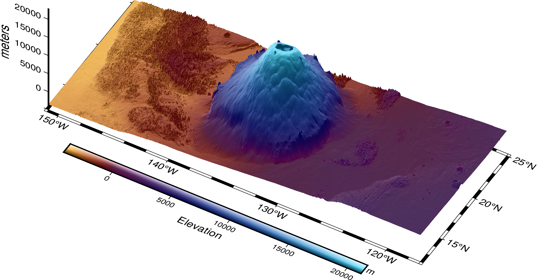
1️⃣ Using grdview for 3-D Visualization#
The grdview
method in PyGMT is a powerful tool for creating 3-D perspective views of gridded data.
By adjusting azimuth and elevation parameters, you can change the viewpoint, helping you
to highlight specific terrain features or data patterns. Let’s go through how these
parameters affect the visualization.
Setting the Perspective: Azimuth and Elevation
Azimuth (
azimuth): Controls the horizontal rotation of the view, ranging from 0° to 360°. Lower values (close to 0°) represent a viewpoint from the north, while 90° gives a view from the east, 180° from the south, and 270° from the west. Experimenting with azimuth can help showcase specific aspects of the data from different angles.Elevation (
elevation): Controls the vertical angle of the view, with 90° representing a top-down perspective and lower values providing more of a side view. Typically, values between 20° and 60° create a balanced 3-D effect.
Example: Using perspective=[150, 45] means azimuth=150 and elevation=45, which
gives you a southeast view, tilted at a moderate angle to capture both horizontal and
vertical details.
fig = pygmt.Figure()

fig.grdview(
    grid=da_olympus,
    cmap="SCM/managua+h0",
    region=[-151, -117, 12, 25, -5000, 23000],  # xmin, xmax, ymin, ymax, zmin, zmax
    projection="M12c",
    perspective=[150, 45],  # azimuth bearing, and elevation angle
    zsize="4c",  # vertical exaggeration
    surftype="s",  # surface plot
    shading=True,
    frame=["xaf", "yaf", "z5000+lmeters"],
)

fig.colorbar(frame=["a5000", "x+lElevation", "y+lm"], perspective=True, shading=True)
fig.show()
Note that there are other things we have configured such as:
zsize - vertical exaggeration as z-axis size, we used
4chere for 4 centimeterssurftype - using
swill just create a regular surfaceshading - set to
Trueto get the default hillshading effectframe - A proper 3-D map frame that consists of:
automatic tick marks on x and y axis (e.g.,
xafandyaf)z-axis tick marks every 5000m, plus a label (
z5000+lLabel)
Tip
When choosing azimuth and elevation, always consider how the scene is illuminated. Azimuth angles that align with typical light directions (e.g., from the northwest) often provide the most natural and visually appealing shadows. Elevations between 20° and 45° typically create a good balance, highlighting terrain features without flattening or obscuring them. You can experiment with different combinations to best reveal the data’s structure.
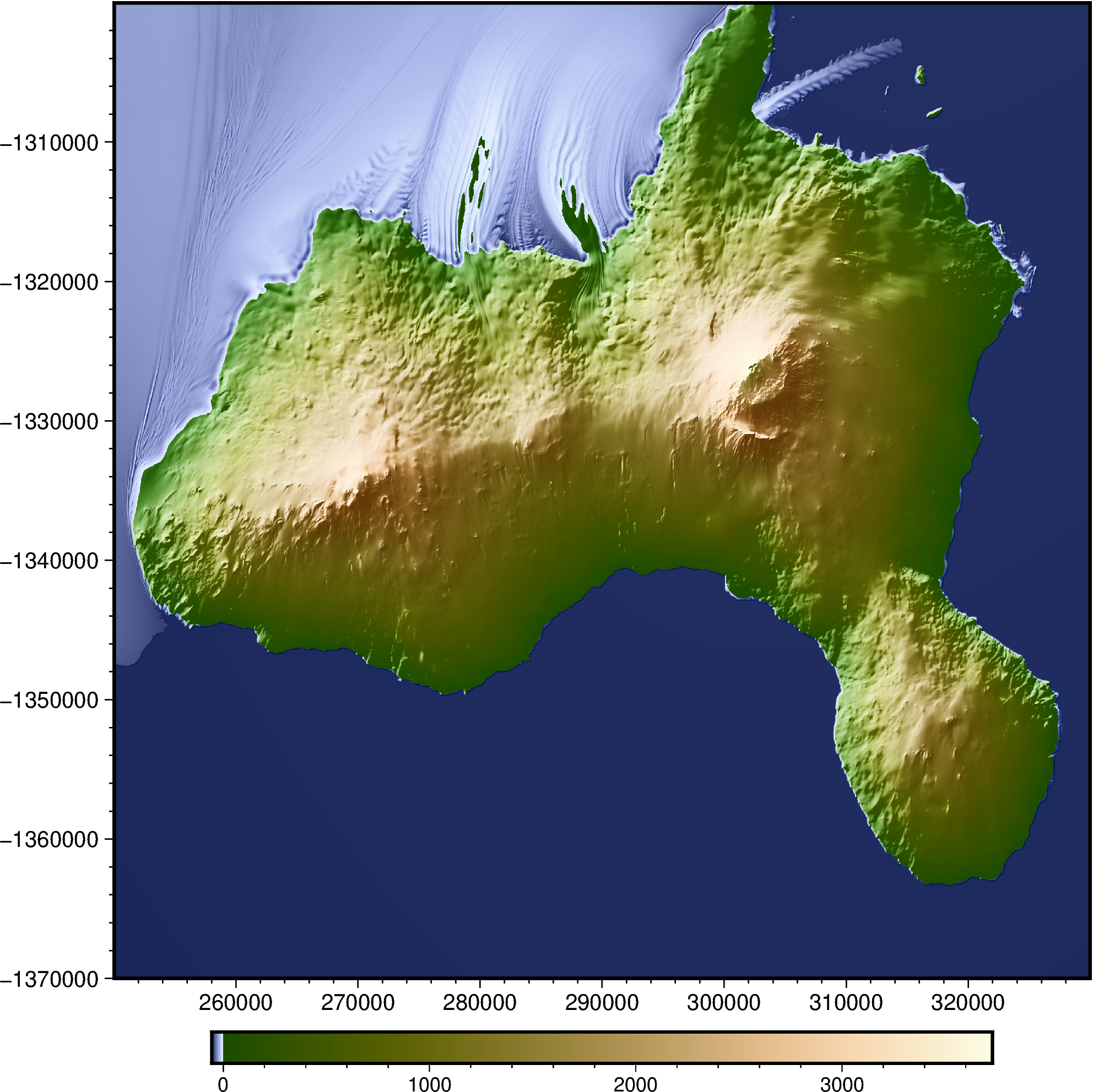
2️⃣ Antarctic Digital Elevation Model#
For the next exercise, we’ll pay a visit to the Antarctic continent, specifically, looking at Ross Island where the McMurdo Station (US) and Scott Base (NZ) is located. We’ll learn how to drape some RGB imagery from Sentinel-2 onto some DEM tiles from the Reference Elevation Model of Antarctica (REMA).
🔖 References:
Howat et al. [2019]
2.1 Getting a DEM mosaic#
The REMA tiles are distributed as several GeoTIFF files. Our area of interest over Ross Island spans two tiles, so we’ll need to retrieve them both an mosaic them. There are several sources for REMA, but we’ll use one sourced from https://registry.opendata.aws/pgc-rema/. The two specific tiles we’ll get can be previewed at:
Tip
To find the tile number, go to https://rema.apps.pgc.umn.edu/ and zoom/pan to the area on the map you’re interested in getting a DEM for. Click on the ‘Identify’ button on the bottom left, and a pop-up will tell you the tile ID number.
To open the GeoTIFF files, we can use
rioxarray.open_rasterio
which load the data into an xarray.DataArray.
tile_17_33 = rioxarray.open_rasterio(
    filename="https://pgc-opendata-dems.s3.us-west-2.amazonaws.com/rema/mosaics/v2.0/32m/17_33/17_33_32m_v2.0_dem.tif"
)
tile_17_34 = rioxarray.open_rasterio(
    filename="https://pgc-opendata-dems.s3.us-west-2.amazonaws.com/rema/mosaics/v2.0/32m/17_34/17_34_32m_v2.0_dem.tif"
)
Next, we’ll use
rioxarray.merge.merge_arrays
to mosaic the two tiles together, and clip it to the spatial extent of Ross Island.
dem_mosaic = rioxarray.merge.merge_arrays(
    dataarrays=[tile_17_33, tile_17_34],
    bounds=(250_000, -1_370_000, 330_000, -1_300_000),  # xmin, ymin, xmax, ymax
).isel(band=0)
Preview the DEM using
pygmt.Figure.grdimage
fig = pygmt.Figure()
fig.grdimage(grid=dem_mosaic, cmap="oleron", frame=True, shading=True)
fig.colorbar()
fig.show()
2.2 Getting RGB imagery#
Next, let’s get some Sentinel-2 optical satellite imagery, which we’ll use to drape on top of the DEM later. We’ll find some relatively cloud-free imagery that was taken on 31 Oct 2024, specifically these ones that can be previewed at:
Tip
There are several online viewers based on Spatiotemporal Asset Catalog (STAC) APIs that allow you to search for satellite imagery. Some examples used here were:
We’ll use rioxarray again to open the GeoTIFF files (using overview_level=1 means
we can get a lower resolution version), and to mosaic the two image tiles together.
tile_58CEU = rioxarray.open_rasterio(
    filename="https://sentinel-cogs.s3.us-west-2.amazonaws.com/sentinel-s2-l2a-cogs/58/C/EU/2024/11/S2B_58CEU_20241109_0_L2A/TCI.tif",
    overview_level=1,
)
tile_58CEV = rioxarray.open_rasterio(
    filename="https://sentinel-cogs.s3.us-west-2.amazonaws.com/sentinel-s2-l2a-cogs/58/C/EV/2024/11/S2B_58CEV_20241109_0_L2A/TCI.tif",
    overview_level=1,
)

rgb_mosaic = rioxarray.merge.merge_arrays(dataarrays=[tile_58CEU, tile_58CEV])
rgb_image = rgb_mosaic.rio.reproject_match(match_data_array=dem_mosaic)
rgb_image
<xarray.DataArray (band: 3, y: 2188, x: 2500)> Size: 16MB
array([[[255, 255, 255, ..., 255, 255, 255],
        [255, 255, 255, ..., 255, 255, 255],
        [255, 255, 255, ..., 255, 255, 255],
        ...,
        [  0,   0,   0, ..., 255, 255, 255],
        [  0,   0,   0, ..., 255, 255, 255],
        [  0,   0,   0, ..., 255, 252, 254]],

       [[255, 255, 255, ..., 255, 255, 255],
        [255, 255, 255, ..., 255, 255, 255],
        [255, 255, 255, ..., 255, 255, 255],
        ...,
        [  0,   0,   0, ..., 255, 255, 255],
        [  0,   0,   0, ..., 255, 255, 255],
        [  0,   0,   0, ..., 255, 255, 255]],

       [[255, 255, 255, ..., 255, 255, 255],
        [255, 255, 255, ..., 255, 255, 255],
        [255, 255, 255, ..., 255, 255, 255],
        ...,
        [  0,   0,   0, ..., 255, 255, 255],
        [  0,   0,   0, ..., 255, 255, 255],
        [  0,   0,   0, ..., 255, 255, 255]]], dtype=uint8)
Coordinates:
  * band         (band) int64 24B 1 2 3
    spatial_ref  int64 8B 0
  * x            (x) float64 20kB 2.5e+05 2.5e+05 2.501e+05 ... 3.3e+05 3.3e+05
  * y            (y) float64 18kB -1.3e+06 -1.3e+06 ... -1.37e+06 -1.37e+06
Attributes:
    OVR_RESAMPLING_ALG:  AVERAGE
    AREA_OR_POINT:       Area
    scale_factor:        1.0
    add_offset:          0.0
_FillValue: 0Tip
When working with DEM mosaics and optical imagery, carefully consider the size and resolution of the data. High-resolution DEMs combined with complex topographies can demand substantial computational resources for processing and visualization. A practical tip is to start with lower resolutions to experiment with and refine the scene geometry (e.g., azimuth, elevation, and perspective). Once you are satisfied with the visualization setup, switch to higher-resolution data for the final rendering. This approach helps optimize computational efficiency while maintaining the quality of your analysis.
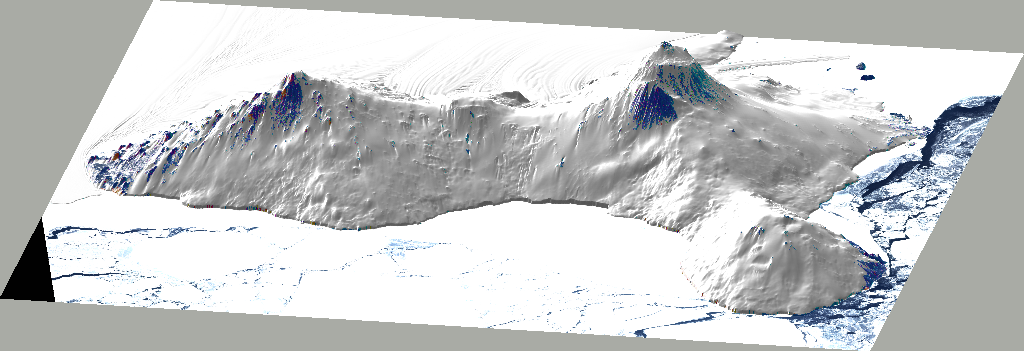
3️⃣ Draping RGB image on 3-D topography#
We have our RGB imagery from Sentinel-2, and a DEM from REMA, and now we can learn how
to render the color image on top of the 3-D topography! Once again, we will be using
grdview, but
pass in some extra arguments:
drapegrid: This is the image that will be overlaid on top of the relief grid.
surftype: We are plotting an RGB image with 3-bands, so we will use
ifor an image plot. It is also possible to append a number (e.g.600) as the dots-per-unit resolution for the rasterizationzscale: vertical exaggeration factor, usually given as a fractional number.
Tip
When setting the zscale for vertical exaggeration, choose a value that balances
clarity and realism. For subtle topographies, higher exaggeration (e.g., smaller
zscale values) can emphasize elevation differences, making features more visible.
However, for steep terrains, lower exaggeration helps maintain a natural appearance. You
may use shading=True to add hillshading, which enhances the 3-D effect by simulating
light and shadows, making terrain features easier to interpret. Experiment with both
parameters to find the best combination for your dataset and visualization goals.
This is how the code will look like. We’ll also use
pygmt.config to set
PS_PAGE_COLOR
(the background color) to an off-white color instead of the default black to better
match the polar landscape.
fig = pygmt.Figure()
with pygmt.config(PS_PAGE_COLOR="#a9aba5"):
    fig.grdview(
        grid=dem_mosaic,  # DEM layer
        drapegrid=rgb_image,  # Sentinel-2 image layer
        surftype="i600",  # image draping with 600dpi resolution
        perspective=[170, 20],  # view azimuth and angle
        zscale="0.0005",  # vertical exaggeration
        shading=True,  # hillshading
        # frame="af",
    )
fig.show()
grdview [WARNING]: (w - x_min) must equal (NX + eps) * x_inc), where NX is an integer and |eps| <= 0.0001.
grdview [WARNING]: w reset from 250016 to 250000
grdview [WARNING]: (e - x_min) must equal (NX + eps) * x_inc), where NX is an integer and |eps| <= 0.0001.
grdview [WARNING]: e reset from 329984 to 330000
grdview [WARNING]: (s - y_min) must equal (NY + eps) * y_inc), where NY is an integer and |eps| <= 0.0001.
grdview [WARNING]: s reset from -1370000 to -1370016
grdview [WARNING]: (n - y_min) must equal (NY + eps) * y_inc), where NY is an integer and |eps| <= 0.0001.
grdview [WARNING]: n reset from -1300016 to -1300000
See also
Examples of other 3D perspective plots made with PyGMT:
References
Ian M. Howat, Claire Porter, Benjamin E. Smith, Myoung-Jong Noh, and Paul Morin. The Reference Elevation Model of Antarctica. The Cryosphere, 13(2):665–674, February 2019. doi:10.5194/tc-13-665-2019.
G. A. Neumann, J. B. Abshire, O. Aharonson, J. B. Garvin, X. Sun, and M. T. Zuber. Mars Orbiter Laser Altimeter pulse width measurements and footprint-scale roughness. Geophysical Research Letters, 30(11):2003GL017048, June 2003. doi:10.1029/2003GL017048.