LiDAR Point clouds to 3D surfaces ✨➡️🏔️¶

In this tutorial, let’s use PyGMT to perform a more advanced geoprocessing workflow 😎

Specifically, we’ll learn to filter and interpolate a LiDAR point cloud onto a regular grid surface 🏁

At the end, we’ll also make a 🚠 3D perspective plot for the Digital Surface Model (DSM) produced through this exercise!

🎉 Getting started¶

Begin by importing some Python 🐍 libraries.

Besides pygmt, we’ll also be using:

laspy to read in LAZ LiDAR files 🌃
pandas for managing tabular data 🀤
rioxarray to export our DSM to a GeoTIFF 🗺️

import laspy
import pandas as pd
import pygmt
import rioxarray
import xarray as xr

0️⃣ The LiDAR data¶

Let’s visit Wellington which is the capital city of New Zealand 🇳🇿.

They recently had a LiDAR survey done between March 2019 to March 2020 🛩️, with the point cloud and derived products published under an open CC BY 4.0 license.

OpenTopography link: https://doi.org/10.5069/G9K935QX
Bulk download location: https://opentopography.s3.sdsc.edu/minio/pc-bulk/NZ19_Wellington
Official 1m DSM from LINZ: https://data.linz.govt.nz/layer/105024-wellington-city-lidar-1m-dsm-2019-2020

🔖 References:

First though, we’ll need to download a sample file to play with 🎮

Luckily for us, there is a function called pygmt.which that has to ability to do just that!

The download=True option can be used to download ⬇️ a remote file to our local working directory.

# Download LiDAR LAZ file from a URL
lazfile = pygmt.which(
    fname="https://opentopography.s3.sdsc.edu/pc-bulk/NZ19_Wellington/CL2_BQ31_2019_1000_2138.laz",
    download=True,
)
print(lazfile)

CL2_BQ31_2019_1000_2138.laz

Loading a point cloud 🌧️¶

Now we can use laspy to read in our example LAZ file into a pandas.DataFrame.

The data will be kept in a variable called ‘df’ which stands for dataframe.

# Load LAZ data into a pandas DataFrame
lazdata = laspy.read(source=lazfile)
df = pd.DataFrame(
    data={
        "x": lazdata.x.scaled_array(),
        "y": lazdata.y.scaled_array(),
        "z": lazdata.z.scaled_array(),
        "classification": lazdata.classification,
    }
)

Quick data preview ⚡¶

Let’s get the bounding box 📦 region of our study area using pygmt.info.

# Get bounding box region
region = pygmt.info(data=df[["x", "y"]], spacing=1)  # West, East, South, North
print(f"Data points covers region: {region}")

Data points covers region: [1749760. 1750240. 5426880. 5427600.]

Check how many 🗃️ data points (rows) are in the table and get some summary statistics printed out.

# Print summary statistics
print(f"Total of {len(df)} data points")
df.describe()

Total of 7322702 data points

	x	y	z	classification
count	7.322702e+06	7.322702e+06	7.322702e+06	7.322702e+06
mean	1.750009e+06	5.427144e+06	6.536329e+01	4.477295e+00
std	1.337038e+02	1.713325e+02	4.428189e+01	2.212308e+00
min	1.749760e+06	5.426880e+06	-1.377360e+02	1.000000e+00
25%	1.749896e+06	5.426997e+06	3.380700e+01	3.000000e+00
50%	1.750012e+06	5.427125e+06	6.012200e+01	5.000000e+00
75%	1.750121e+06	5.427280e+06	9.645000e+01	5.000000e+00
max	1.750240e+06	5.427600e+06	3.186180e+02	1.800000e+01

More than 7 million points, that’s a lot! 🤯

Let’s try to take a quick look of our LiDAR elevation points on a map 🗺️

PyGMT can plot these many points, but it might take a long time ⏳, so let’s do a quick filter by taking every n-th row from our dataframe table.

df_filtered = df.iloc[::20]
print(f"Filtered down to {len(df_filtered)} data points")

Filtered down to 366136 data points

Now we can visualize these quickly on a map with PyGMT 😀

# Plot XYZ points on a map
fig = pygmt.Figure()
fig.basemap(frame=True, region=region, projection="x1:5000")
pygmt.makecpt(cmap="bukavu", series=[df.z.min(), df.z.max()])
fig.plot(
    x=df_filtered.x, y=df_filtered.y, color=df_filtered.z, style="c0.03c", cmap=True
)
fig.colorbar(position="JMR", frame=["af+lElevation", "y+lm"])
fig.show()

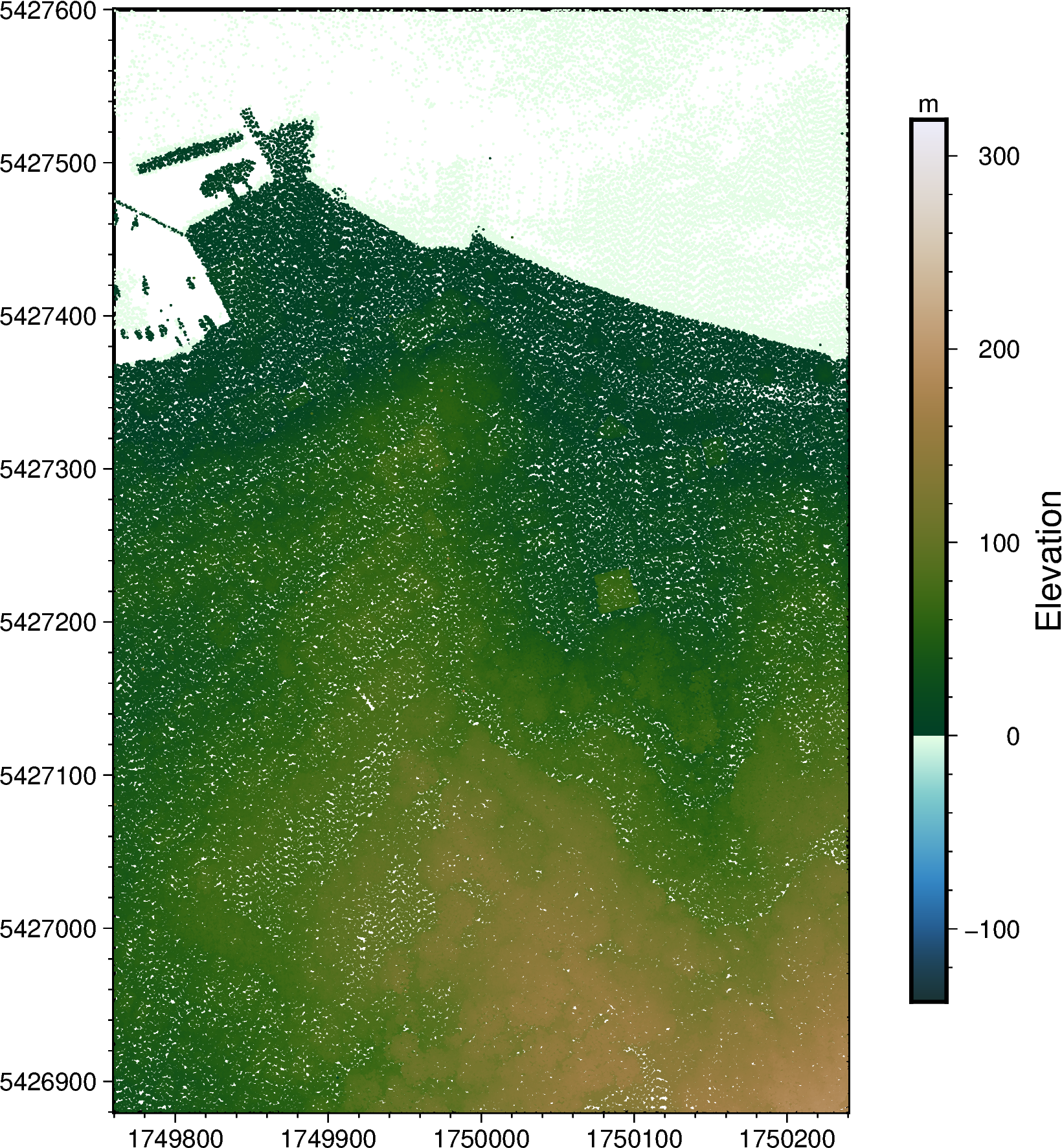
It’s hard to make out what the objects are, but hopefully you’ll see what looks like a wharf with ⛵ boats on the top left corner.

This is showing us a part of Oriental Bay in Wellington, with Mount Victoria ⛰️ towards the Southeast corner of the map.

1️⃣ Creating a Digital Surface Model (DSM)¶

Let’s now produce a digital surface model from our point cloud 🌧️

We’ll first do some proper spatial data cleaning 🧹 using both pandas and pygmt.

First step is to remove the LiDAR points classified as high noise 🔊 which is done by querying all the points that are not ‘18’.

🔖 References:

Table 17 of ASPRS LAS Specification

df = df.query(expr="classification != 18")
df

	x	y	z	classification
0	1749771.56	5427498.77	-0.724	2
1	1749771.52	5427498.46	-0.708	2
2	1749771.48	5427498.15	-0.700	2
3	1749771.45	5427497.84	-0.683	2
4	1749771.41	5427497.54	-0.630	2
...	...	...	...	...
7322687	1749760.95	5427567.17	-0.479	9
7322698	1749760.23	5427567.65	-0.488	9
7322699	1749760.26	5427567.98	-0.442	9
7322700	1749760.29	5427568.29	-0.417	9
7322701	1749760.32	5427568.62	-0.404	9

7232453 rows × 4 columns

Get highest elevation points 🍫¶

Next, we’ll use the blockmedian function to trim 🪒 down the points spatially.

By default, this function computes a single median elevation for every pixel on an equally spaced grid 🏁

For a Digital Surface Elevation Model (DSM) though, we should pick the highest elevation 🔝 instead of the median.

So we’ll tell blockmedian to use the 99th quantile (T) instead, and set our output grid spacing to be exactly 1 metre (1+e) 📏

Note that we’ll only be taking the 🇽, 🇾, 🇿 (elevation) columns for this.

# Preprocess LiDAR data using blockmedian
df_trimmed = pygmt.blockmedian(
    data=df[["x", "y", "z"]],
    T=0.99,  # 99th quantile, i.e. the highest point
    spacing="1+e",
    region=region,
)
df_trimmed

	x	y	z
0	1749760.05	5427599.54	-0.755
1	1749760.67	5427599.83	-0.737
2	1749761.87	5427599.71	-0.747
3	1749765.39	5427599.55	-0.701
4	1749765.96	5427599.73	-0.742
...	...	...	...
311584	1750236.41	5426880.41	178.756
311585	1750237.32	5426880.47	179.132
311586	1750238.50	5426880.40	179.232
311587	1750239.36	5426880.46	179.517
311588	1750239.99	5426880.49	179.622

311589 rows × 3 columns

2️⃣ Plotting a Digital Surface Model (DSM)¶

Plot in 2D 🏳️‍🌈¶

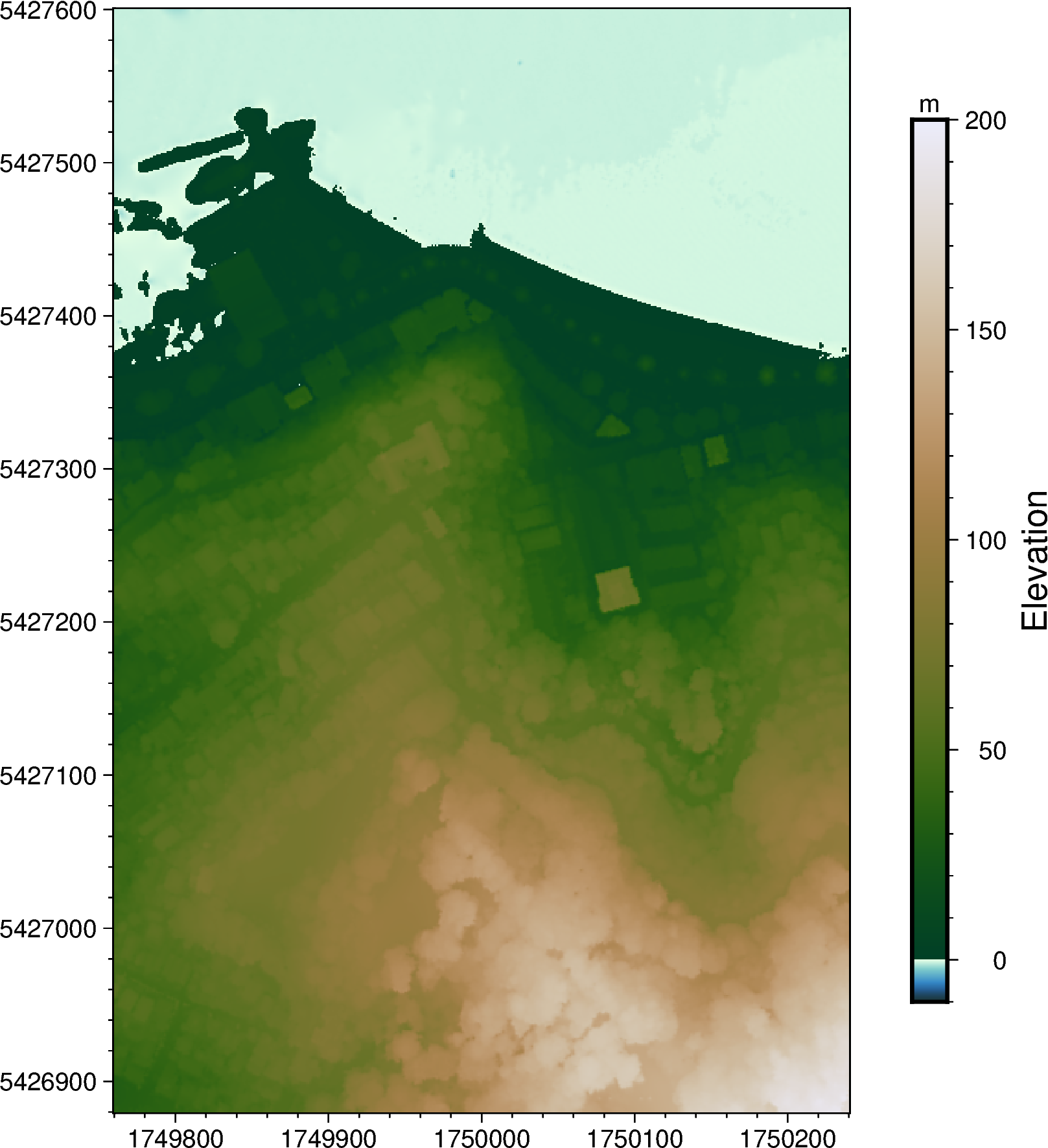
Now we can plot our Digital Surface Model (DSM) grid 🏁

This can be done by passing the xarray.DataArray grid into pygmt.Figure.grdimage.

fig2 = pygmt.Figure()
fig2.basemap(
    frame=True,
    region=[1_749_760, 1_750_240, 5_426_880, 5_427_600],
    projection="x1:5000",
)
pygmt.makecpt(cmap="bukavu", series=[-10, 200])
fig2.grdimage(grid=grid, cmap=True)
fig2.colorbar(position="JMR", frame=["af+lElevation", "y+lm"])
fig2.show()

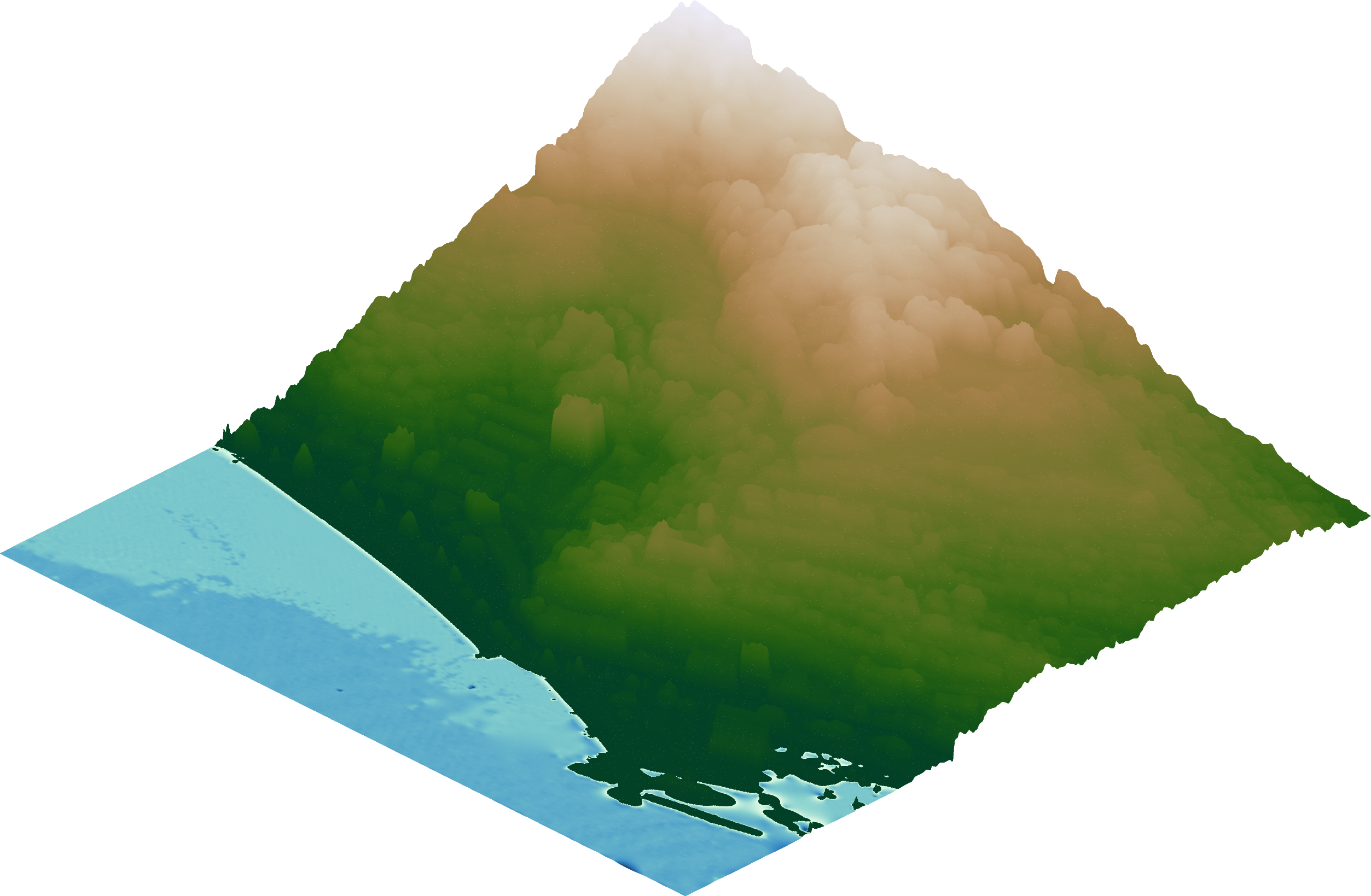
Plot 3D perspective view ⛰️¶

Now comes the cool part 💯

PyGMT has a grdview function to make high quality 3D perspective plots of our elevation surface!

Besides providing the elevation ‘grid’, there are a few basic things to configure:

cmap - name of 🌈 colormap to use
surftype - we’ll use ‘s’ here which just creates a regular surface 🏄
perspective - set azimuth angle (e.g. 315 for NorthWest) and 📐 elevation (e.g 30 degrees) of the viewpoint
zscale - a vertical exaggeration 🔺 factor, we’ll use 0.02 here

fig3 = pygmt.Figure()
fig3.grdview(
    grid=grid,
    cmap="bukavu",
    surftype="s",  # surface plot
    perspective=[315, 30],  # azimuth bearing, and elevation angle
    zscale=0.02,  # vertical exaggeration
)
fig3.show()

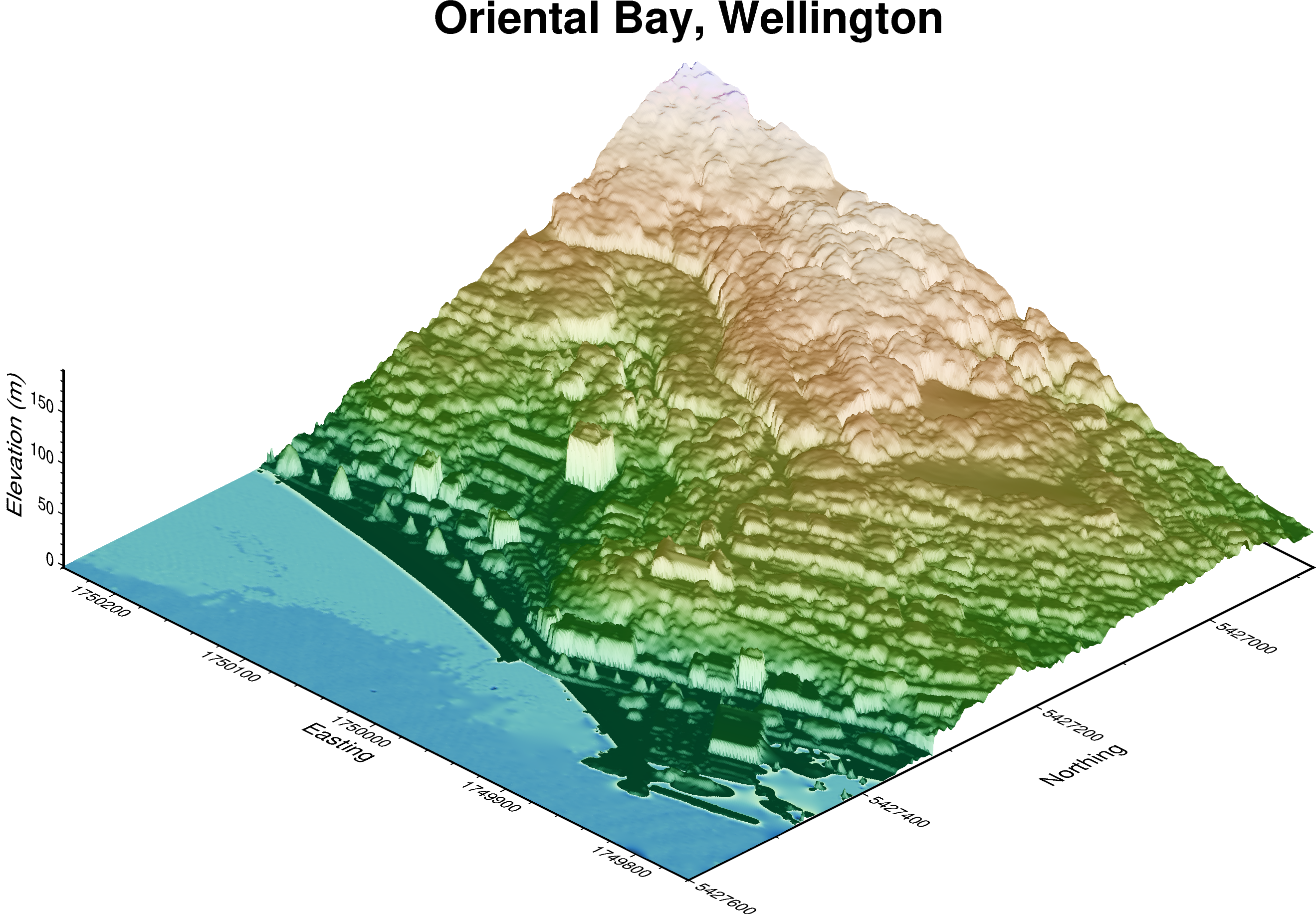
There are also other things we can 🧰 configure such as:

Hillshading ⛱️ using shading=True
A proper 3D map frame 🖼️ with:
- automatic tick marks on x and y axis (e.g. xaf+lLabel)
- z-axis automatic tick marks (zaf+lLabel)
- plot title (+tMy Title)

fig3 = pygmt.Figure()
fig3.grdview(
    grid=grid,
    cmap="bukavu",
    surftype="s",  # surface plot
    perspective=[315, 30],  # azimuth bearing, and elevation angle
    zscale=0.02,  # vertical exaggeration
    shading=True,  # hillshading
    frame=[
        "xaf+lEasting",
        "yaf+lNorthing",
        "zaf+lElevation (m)",
        "+tOriental Bay, Wellington",
    ],
)
fig3.show()

Feel free to have a go at changing the azimuth and elevation angle to get a different view 🔭

You can also try to tweak the vertical exaggeration factor 🗼 and play around with the map frame!

Save figures and output DSM to GeoTIFF 💾¶

Time to save your work!

We’ll save each of our figures into separate files first 🗃️

fig.savefig(fname="wellington_1d_lidar.png")
fig2.savefig(fname="wellington_2d_dsm_map.png")
fig3.savefig(fname="wellington_3d_dsm_view.png")

Also, it’ll be good to have a proper GeoTIFF of the DSM we made. This can be done using rioxarray’s to_raster method.

grid.rio.to_raster(raster_path="DSM_of_Wellington.tif")

---------------------------------------------------------------------------
AttributeError                            Traceback (most recent call last)
Cell In[16], line 1
----> 1 grid.rio.to_raster(raster_path="DSM_of_Wellington.tif")

File /usr/share/miniconda3/envs/egu22pygmt/lib/python3.9/site-packages/rioxarray/raster_array.py:1100, in RasterArray.to_raster(self, raster_path, driver, dtype, tags, windowed, recalc_transform, lock, compute, **profile_kwargs)
out_profile = {
   key: value
   for key, value in out_profile.items()
   (...)
   )
}
rio_nodata = (
   self.encoded_nodata if self.encoded_nodata is not None else self.nodata
)
-> 1100 return RasterioWriter(raster_path=raster_path).to_raster(
   xarray_dataarray=self._obj,
   tags=tags,
   driver=driver,
   height=int(self.height),
   width=int(self.width),
   count=int(self.count),
   dtype=dtype,
   crs=self.crs,
   transform=self.transform(recalc=recalc_transform),
   gcps=self.get_gcps(),
   nodata=rio_nodata,
   windowed=windowed,
   lock=lock,
   compute=compute,
   **out_profile,
)

File /usr/share/miniconda3/envs/egu22pygmt/lib/python3.9/site-packages/rioxarray/raster_writer.py:252, in RasterioWriter.to_raster(self, xarray_dataarray, tags, windowed, lock, compute, **kwargs)
else:
   out_data = xarray_dataarray
--> 252 data = encode_cf_variable(out_data).values.astype(numpy_dtype)
if data.ndim == 2:
   rds.write(data, 1, window=window)

File /usr/share/miniconda3/envs/egu22pygmt/lib/python3.9/site-packages/xarray/conventions.py:296, in encode_cf_variable(var, needs_copy, name)
ensure_not_multiindex(var, name=name)
for coder in [
   times.CFDatetimeCoder(),
   times.CFTimedeltaCoder(),
   (...)
   variables.UnsignedIntegerCoder(),
]:
--> 296     var = coder.encode(var, name=name)
# TODO(shoyer): convert all of these to use coders, too:
var = maybe_encode_nonstring_dtype(var, name=name)

File /usr/share/miniconda3/envs/egu22pygmt/lib/python3.9/site-packages/xarray/coding/times.py:690, in CFDatetimeCoder.encode(self, variable, name)
def encode(self, variable: Variable, name: T_Name = None) -> Variable:
   if np.issubdtype(
       variable.data.dtype, np.datetime64
--> 690     ) or contains_cftime_datetimes(variable):
       dims, data, attrs, encoding = unpack_for_encoding(variable)
       (data, units, calendar) = encode_cf_datetime(
           data, encoding.pop("units", None), encoding.pop("calendar", None)
       )

File /usr/share/miniconda3/envs/egu22pygmt/lib/python3.9/site-packages/xarray/core/common.py:1818, in contains_cftime_datetimes(var)
def contains_cftime_datetimes(var: T_Variable) -> bool:
   """Check if an xarray.Variable contains cftime.datetime objects"""
-> 1818     return _contains_cftime_datetimes(var._data)

File /usr/share/miniconda3/envs/egu22pygmt/lib/python3.9/site-packages/xarray/core/common.py:276, in AttrAccessMixin.__getattr__(self, name)
       with suppress(KeyError):
           return source[name]
--> 276 raise AttributeError(
   f"{type(self).__name__!r} object has no attribute {name!r}"
)

AttributeError: 'DataArray' object has no attribute '_data'

The files should now appear on the file list on the left, and you can download them to your computer.

3️⃣ Bonus exercise - Create a 3D surface map of another area¶

Here’s a challenge to test your PyGMT skills 🤹

You’ll be processing a LiDAR point cloud of a different area 📍 from start to finish.

Good luck! 🥳

Feel free to find a dataset from an area you’re interested in using OpenTopography.

To make it easier though, I’ve provided an example for Queenstown, New Zealand 🇳🇿

OpenTopography link: https://doi.org/10.5069/G9MP51G0
Bulk download location: https://opentopography.s3.sdsc.edu/minio/pc-bulk/NZ21_Otago
Official 1m DSM from LINZ: https://data.linz.govt.nz/layer/105905-otago-queenstown-lidar-index-tiles-2021

These files covers the Central Queenstown area:

Download and load data¶

filenames = [
    # "",
]

df = pd.DataFrame()  # Start an empty DataFrame
for fname in filenames:
    lazfile = pygmt.which(fname=fname, download=True)

    lazdata = laspy.read(source=lazfile)
    temp_df = pd.DataFrame(
        data={
            "x": lazdata.x.scaled_array(),
            "y": lazdata.y.scaled_array(),
            "z": lazdata.z.scaled_array(),
            "classification": lazdata.classification,
        }
    )
    # load each point cloud into the DataFrame
    df = df.append(temp_df, ignore_index=True)

df

Create a DSM¶

# Run blockmedian

# Run surface

Plot the DSM¶

# Run grdimage

# Run grdview

That’s all 🎉! For more information on how to customize your map 🗺️, check out:

Tutorials at https://www.pygmt.org/v0.6.1/tutorials/index.html
Gallery examples at https://www.pygmt.org/v0.6.1/gallery/index.html

If you have any questions 🙋, feel free to visit the PyGMT forum at https://forum.generic-mapping-tools.org/c/questions/pygmt-q-a/11.

Submit any ✨ feature requests/bug reports to the GitHub repo at https://github.com/GenericMappingTools/pygmt

Cheers!

Crafting beautiful maps with PyGMT

LiDAR Point clouds to 3D surfaces ✨➡️🏔️

Contents