Making some Mars maps with pygmt¶

This tutorial page covers the basics of creating some maps and 3D plot of Mars (yes! Mars). The idea here is to demonstrate that you can use a simple sequence of commands with PyGMT, a Python wrapper for the Generic Mapping Tools (GMT), and with some public data about the topography of Mars, create your own maps, as well as compare this topography with what we know of our own planet Earth.

Mars dataset¶

First, we open the mola32.nc file using xarray. Note the longitudes are from 0-360°, latitudes are distributed from North to South and the alt variable is the MOLA Topography at 32 pixels/degree built from original MOLA file megt90n000fb.img. The source is the Mars Climate Database from the European Space Agency.

# Also, if you are in colab or trying from your jupyter, you will need the Mars Topography (MOLA) already in Netcdf
# a copy of the original file distributed from the Mars Climate Database,
# from the European Space Agency under ESTEC contract 11369/95/NL/JG(SC) and Centre National D'Etude Spatial
# is on GitHub.

!wget https://github.com/andrebelem/PlanetaryMaps/raw/v1.0/mola32.nc

Just like any other notebook with pygmt, we import the library and manipulate other data. To make a map of the entire Martian surface without a lot of time and memory, let’s reduce the resolution using grdsample. We also take the opportunity to transform an alt variable into a float to be used in maps.

import pygmt

dset_mars_topo = dset_mars.alt.astype(float)
dset_mars_topo = pygmt.grdsample(grid=dset_mars_topo, translate=True, spacing=[1,1])

grdsample [WARNING]: (x_max-x_min) must equal (NX + eps) * x_inc), where NX is an integer and |eps| <= 0.0001.

grdsample [WARNING]: (y_max-y_min) must equal (NY + eps) * y_inc), where NY is an integer and |eps| <= 0.0001.

grdsample (gmtapi_init_grdheader): Please select compatible -R and -I values

grdsample [WARNING]: Output sampling interval in x exceeds input interval and may lead to aliasing.

grdsample [WARNING]: Output sampling interval in y exceeds input interval and may lead to aliasing.

Here we can create a map of the entire Martian surface, in the same projections we use for our planet.

fig = pygmt.Figure()

fig.grdimage(grid=dset_mars_topo,region='g',frame=True,projection='W12c')
fig.colorbar(frame=['a5000','x+lElevation','y+lm'])

fig.show()

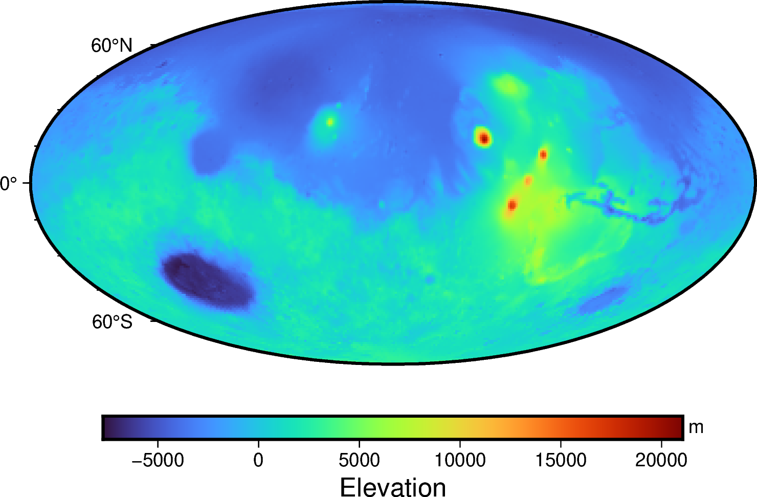
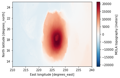
A very interesting feature is Mount Olympus (Olympus Mons - see more details at https://mars.nasa.gov/resources/22587/olympus-mons), centered at approximately 19°N and 133°W, with a height of 22 km (14 miles) and approximately 700 km (435 miles) in diameter. Let’s use the original dataset at 32 pixels/degree resolution and plot a (not so interesting) map with xarray.

dset_olympus = dset_mars.sel(latitude=slice(25,13),longitude=slice(210,240)).alt.astype(float)
dset_olympus.plot()

<matplotlib.collections.QuadMesh at 0x7f8dede911f0>

We use the same sequence as other pygmt tutorial notebooks to make a map.

fig = pygmt.Figure()

fig.grdview(grid=dset_olympus,
           region=[210,240,13,25,-5000,23000],
           surftype='s',
           projection='M12c',
           perspective=[150,45],
           zsize='4c',
           frame=['xa5f1','ya5f1','z5000+lmeters','wSEnZ'],shading='+a50+nt1')

bounds = [[210,13],
         [210,25],
         [240,25],
         [240,13],
         [210,13]]

fig.colorbar(perspective=True,frame=['a5000','x+lElevation','y+lm'])
with fig.inset(position='JTR+w3.5c+o0.2c',margin=0,box=None):
    fig.grdimage(grid=dset_mars_topo,region='g',frame=True,projection='W3.5c')
    fig.plot(bounds, pen='1p,red')

fig.show()

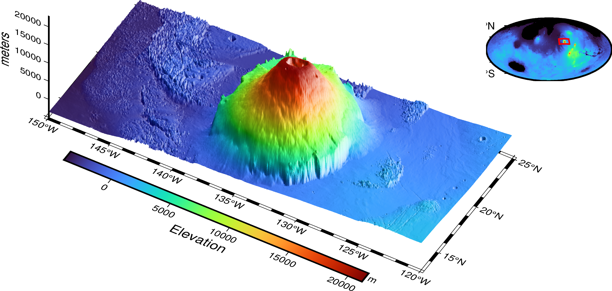
And we’re going to add some perspective, as well as a more interesting color scale. For ease of understanding, let’s separate the region of interest with the same cutout that we created the base of the Olympus Mons topography dataset.

A few notes

zsize is a bit critical here because the volcano is very big (28 km if we consider -5000 to +23000 m). Likewise, perspective=[150,45] was chosen attempting (it’s a matter of taste) and depends of which flank of the volcano you want to show. But this choice has to be made according to shading since to give a good 3D impression, the lighting must be adjusted according to the elevation and azimuth of the perspective. Finally, the pen outline is made smooth and small to enhance the contours of the topography.

Finally, let’s make a combined map showing the planet in an inset in the upper right corner. We use the same bounding box coordinates used to cut out the topography, drawing in red on the map. Obviously here the color scale is the same.

There are a few bonus maps in the extended version in github.

Have fun.

Crafting beautiful maps with PyGMT

Making some Mars maps with pygmt

Contents

Making some Mars maps with pygmt¶

Mars dataset¶