Making some Mars maps with pygmt (extended)¶

This tutorial page covers the basics of creating some maps and 3D plot of Mars (yes! Mars). The idea here is to demonstrate that you can use a simple sequence of commands with PyGMT, a Python wrapper for the Generic Mapping Tools (GMT), and with some public data about the topography of Mars, create your own maps, as well as compare this topography with what we know of our own planet Earth.

first, some options¶

You can run this notebook using your local pygmt installation, or via Binder, or even Google Colaboratory. See comments for each option below.

A) A short note if you are using COLAB

The version of python in COLAB is different from what the newer GMT needs to install along with pygmt. So, one way around this problem is to reinstall GMT from scratch, along with other important packages. This is done with this block of commands below.

comment out the first line of the block (%%script echo skipping) if you want to use colab

%%script echo skipping

# because I like to enjoy my coffee in silence, it takes time.  
# (3 runs averaged 6 minutes to install everything ! keep drinking your coffee)
# comment the %%capture line if you want to see the colab VM working
%%capture
!sudo apt update 
!sudo apt upgrade -y
!sudo apt install -y build-essential cmake libcurl4-gnutls-dev libnetcdf-dev gdal-bin libgdal-dev libfftw3-dev libpcre3-dev liblapack-dev libblas-dev libglib2.0-dev ghostscript ghostscript-x graphicsmagick ffmpeg xdg-utils
# clone gmt from source
!git clone --depth 50 https://github.com/GenericMappingTools/gmt
# cmake everything
!cmake /content/gmt
# build and install
!cmake --build . --target install

# and last but not least
!pip install pygmt

# and if you don't believe in it
!gmt --version
!python --version

skipping

# Also, if you are in colab or trying from your jupyter, you will need the Mars Topography (MOLA) already in Netcdf
# a copy of the original file distributed from the Mars Climate Database,
# from the European Space Agency under ESTEC contract 11369/95/NL/JG(SC) and Centre National D'Etude Spatial
# is in the gdrive.

!gdown 1fDzz8AxR1T58y0IGPhmbb1ZwrTLckp2G

B) Now, if you are using Binder or in your local jupyter

You just skip the block above. Make sure you have the mola32.nc in your folder.

%matplotlib inline

Mars dataset¶

First, we open the mola32.nc file using xarray. Note the longitudes are from 0-360°, latitudes are distributed from North to South and the altvariable is the MOLA Topography at 32 pixels/degree built from original MOLA file megt90n000fb.img.

import xarray as xr 

dset_mars = xr.open_dataset('mola32.nc')
dset_mars

---------------------------------------------------------------------------
KeyError                                  Traceback (most recent call last)
File /usr/share/miniconda3/envs/egu22pygmt/lib/python3.9/site-packages/xarray/backends/file_manager.py:210, in CachingFileManager._acquire_with_cache_info(self, needs_lock)
    209 try:
--> 210     file = self._cache[self._key]
    211 except KeyError:

File /usr/share/miniconda3/envs/egu22pygmt/lib/python3.9/site-packages/xarray/backends/lru_cache.py:56, in LRUCache.__getitem__(self, key)
     55 with self._lock:
---> 56     value = self._cache[key]
     57     self._cache.move_to_end(key)

KeyError: [<class 'netCDF4._netCDF4.Dataset'>, ('/home/runner/work/egu22pygmt/egu22pygmt/book/mola32.nc',), 'r', (('clobber', True), ('diskless', False), ('format', 'NETCDF4'), ('persist', False)), '8cc09da8-2b63-4eea-ac45-1513bd6b58fa']

During handling of the above exception, another exception occurred:

FileNotFoundError                         Traceback (most recent call last)
Cell In[4], line 3
      1 import xarray as xr 
----> 3 dset_mars = xr.open_dataset('mola32.nc')
      4 dset_mars

File /usr/share/miniconda3/envs/egu22pygmt/lib/python3.9/site-packages/xarray/backends/api.py:526, in open_dataset(filename_or_obj, engine, chunks, cache, decode_cf, mask_and_scale, decode_times, decode_timedelta, use_cftime, concat_characters, decode_coords, drop_variables, inline_array, backend_kwargs, **kwargs)
    514 decoders = _resolve_decoders_kwargs(
    515     decode_cf,
    516     open_backend_dataset_parameters=backend.open_dataset_parameters,
   (...)
    522     decode_coords=decode_coords,
    523 )
    525 overwrite_encoded_chunks = kwargs.pop("overwrite_encoded_chunks", None)
--> 526 backend_ds = backend.open_dataset(
    527     filename_or_obj,
    528     drop_variables=drop_variables,
    529     **decoders,
    530     **kwargs,
    531 )
    532 ds = _dataset_from_backend_dataset(
    533     backend_ds,
    534     filename_or_obj,
   (...)
    542     **kwargs,
    543 )
    544 return ds

File /usr/share/miniconda3/envs/egu22pygmt/lib/python3.9/site-packages/xarray/backends/netCDF4_.py:577, in NetCDF4BackendEntrypoint.open_dataset(self, filename_or_obj, mask_and_scale, decode_times, concat_characters, decode_coords, drop_variables, use_cftime, decode_timedelta, group, mode, format, clobber, diskless, persist, lock, autoclose)
    557 def open_dataset(
    558     self,
    559     filename_or_obj,
   (...)
    574     autoclose=False,
    575 ):
    576     filename_or_obj = _normalize_path(filename_or_obj)
--> 577     store = NetCDF4DataStore.open(
    578         filename_or_obj,
    579         mode=mode,
    580         format=format,
    581         group=group,
    582         clobber=clobber,
    583         diskless=diskless,
    584         persist=persist,
    585         lock=lock,
    586         autoclose=autoclose,
    587     )
    589     store_entrypoint = StoreBackendEntrypoint()
    590     with close_on_error(store):

File /usr/share/miniconda3/envs/egu22pygmt/lib/python3.9/site-packages/xarray/backends/netCDF4_.py:382, in NetCDF4DataStore.open(cls, filename, mode, format, group, clobber, diskless, persist, lock, lock_maker, autoclose)
    376 kwargs = dict(
    377     clobber=clobber, diskless=diskless, persist=persist, format=format
    378 )
    379 manager = CachingFileManager(
    380     netCDF4.Dataset, filename, mode=mode, kwargs=kwargs
    381 )
--> 382 return cls(manager, group=group, mode=mode, lock=lock, autoclose=autoclose)

File /usr/share/miniconda3/envs/egu22pygmt/lib/python3.9/site-packages/xarray/backends/netCDF4_.py:329, in NetCDF4DataStore.__init__(self, manager, group, mode, lock, autoclose)
    327 self._group = group
    328 self._mode = mode
--> 329 self.format = self.ds.data_model
    330 self._filename = self.ds.filepath()
    331 self.is_remote = is_remote_uri(self._filename)

File /usr/share/miniconda3/envs/egu22pygmt/lib/python3.9/site-packages/xarray/backends/netCDF4_.py:391, in NetCDF4DataStore.ds(self)
    389 @property
    390 def ds(self):
--> 391     return self._acquire()

File /usr/share/miniconda3/envs/egu22pygmt/lib/python3.9/site-packages/xarray/backends/netCDF4_.py:385, in NetCDF4DataStore._acquire(self, needs_lock)
    384 def _acquire(self, needs_lock=True):
--> 385     with self._manager.acquire_context(needs_lock) as root:
    386         ds = _nc4_require_group(root, self._group, self._mode)
    387     return ds

File /usr/share/miniconda3/envs/egu22pygmt/lib/python3.9/contextlib.py:119, in _GeneratorContextManager.__enter__(self)
    117 del self.args, self.kwds, self.func
    118 try:
--> 119     return next(self.gen)
    120 except StopIteration:
    121     raise RuntimeError("generator didn't yield") from None

File /usr/share/miniconda3/envs/egu22pygmt/lib/python3.9/site-packages/xarray/backends/file_manager.py:198, in CachingFileManager.acquire_context(self, needs_lock)
    195 @contextlib.contextmanager
    196 def acquire_context(self, needs_lock=True):
    197     """Context manager for acquiring a file."""
--> 198     file, cached = self._acquire_with_cache_info(needs_lock)
    199     try:
    200         yield file

File /usr/share/miniconda3/envs/egu22pygmt/lib/python3.9/site-packages/xarray/backends/file_manager.py:216, in CachingFileManager._acquire_with_cache_info(self, needs_lock)
    214     kwargs = kwargs.copy()
    215     kwargs["mode"] = self._mode
--> 216 file = self._opener(*self._args, **kwargs)
    217 if self._mode == "w":
    218     # ensure file doesn't get overridden when opened again
    219     self._mode = "a"

File src/netCDF4/_netCDF4.pyx:2353, in netCDF4._netCDF4.Dataset.__init__()

File src/netCDF4/_netCDF4.pyx:1963, in netCDF4._netCDF4._ensure_nc_success()

FileNotFoundError: [Errno 2] No such file or directory: b'/home/runner/work/egu22pygmt/egu22pygmt/book/mola32.nc'

Just like any other notebook with pygmt, we import the library and manipulate other data. To make a map of the entire Martian surface without a lot of time and memory, let’s reduce the resolution using grdsample. We also take the opportunity to transform an alt variable into a float to be used in maps.

import pygmt 

# convert from int16 to float
dset_mars_topo = dset_mars.alt.astype(float)

# May be a global Mars map is very interesting. We just need to get a better resolution not to consume all memory
# translate here changes from grid to pixel registration and spacing sets to 1 degree resolution
dset_mars_topo = pygmt.grdsample(grid=dset_mars_topo,translate=True,spacing=[1,1])

# don't be worried about the warnings.

Here we can create a map of the entire Martian surface, in the same projections we use for our planet.

fig = pygmt.Figure()

fig.grdimage(grid=dset_mars_topo,region='g',frame=True,projection='Cyl_stere/0/0/12c')
# you can try with different cylindrical or miscellaneous projections
# see at https://www.pygmt.org/dev/projections/index.html
# some ideas: Eckert IV = Kf; Hammer = H; Mollweide = W

fig.colorbar(frame=["a5000", "x+lElevation", "y+lm"])
fig.show()

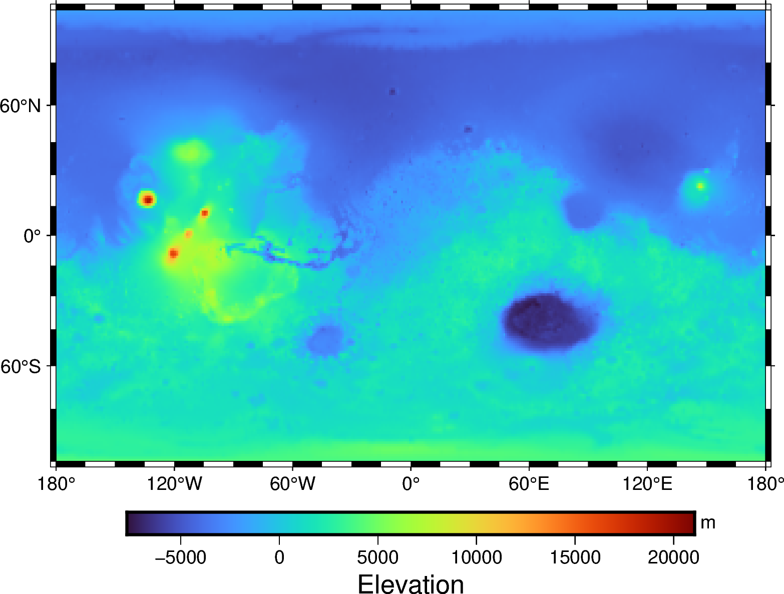
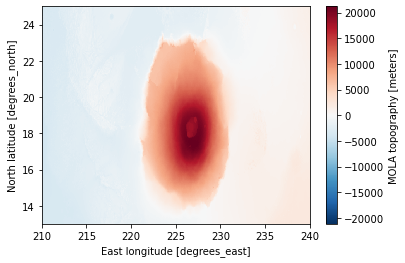
A very interesting feature is Mount Olympus (Olympus Mons - see more details at https://mars.nasa.gov/resources/22587/olympus-mons), centered at approximately 19°N and 133°W, with a height of 22 km (14 miles) and approximately 700 km (435 miles) in diameter. Let’s use the original dataset at 32 pixels/degree resolution and plot a (not so interesting) map with xarray.

# Olympus Mons is located in these slices of 12 degrees of latitude and 30 degrees of longitude
# note we are cutting the region of interest and converting here the original "alt" data in int16 to float (for grid)
dset_olympus = dset_mars.sel(latitude=slice(25,13),longitude=slice(210,240)).alt.astype('float')
dset_olympus.plot()

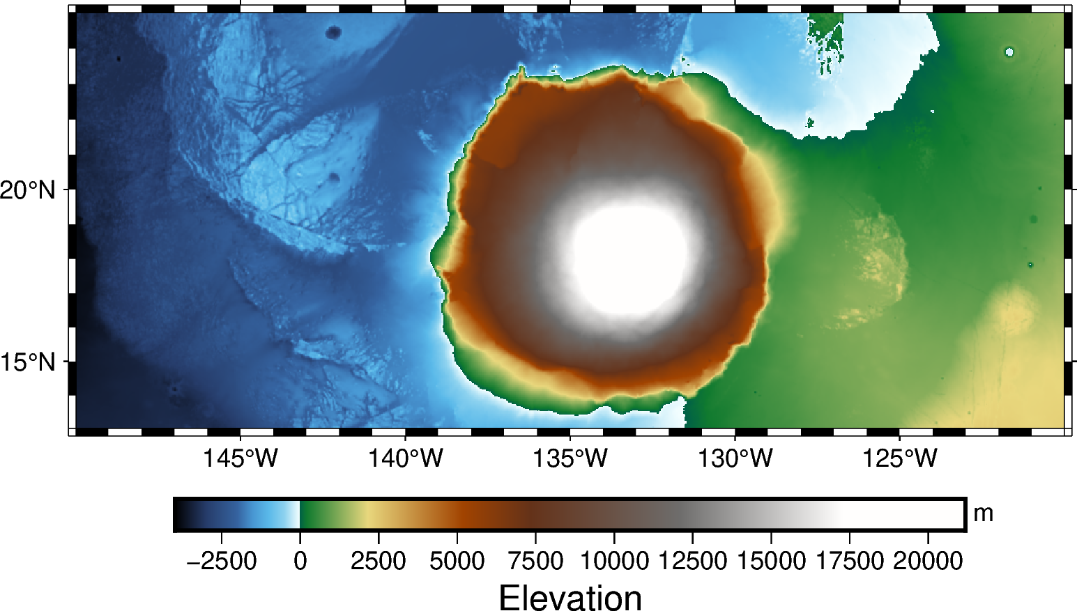
We use the same sequence as other pygmt tutorial notebooks to make a map.

# first things, first
fig = pygmt.Figure()
# note I can add projection, after cmap and after, frame (and control frame)
fig.grdimage(grid=dset_olympus,projection='M12c',frame='a5f1',cmap='geo')
# also, I can add a colorbar (later)
fig.colorbar(frame=["a2500", "x+lElevation", "y+lm"])

fig.show()

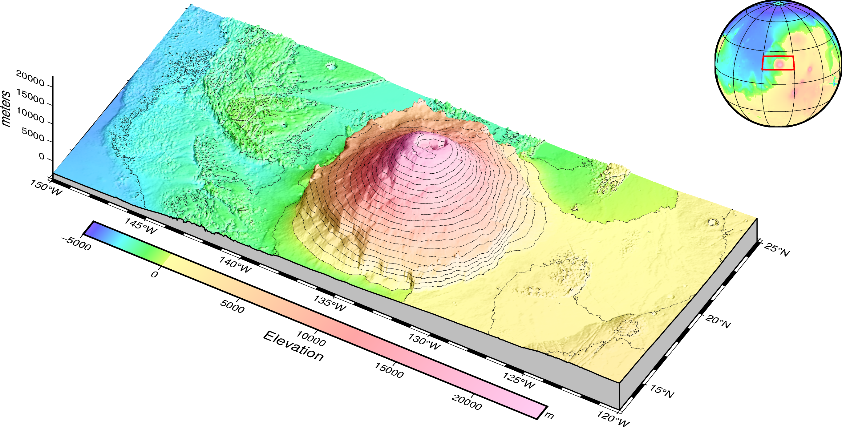
And we’re going to add some perspective, as well as a more interesting color scale. For ease of understanding, let’s separate the region of interest with the same cutout that we created the base of the Olympus Mons topography dataset.

A few notes

zsize is a bit critical here because the volcano is very big (28 km if we consider -5000 to +23000 m). Likewise, perspective=[150.45] was chosen attempting (it’s a matter of taste) and depends of which flank of the volcano you want to show. But this choice has to be made according to shading since to give a good 3D impression, the lighting must be adjusted according to the elevation and azimuth of the perspective. Finally, the pen outline is made smooth and small to enhance the contours of the topography.

Finally, let’s make a combined map showing the planet in an inset in the upper right corner. We use the same bounding box coordinates used to cut out the topography, drawing in red on the map. Obviously here the color scale is the same.

# a little perspective

fig = pygmt.Figure()
# note I can add projection, after cmap and after, frame (and control frame)
topo_cpt = pygmt.makecpt(cmap='sealand',series=f'-5000/24000/1000',continuous=True)
frame =  ["xa5f1","ya5f1", "z5000+lmeters", "wSEnZ"]

fig.grdview(grid=dset_olympus,
            region=[210,240,13,25,-5000,23000],
            frame=frame,
            perspective=[150,45],
            projection='M18c',
            zsize='4c',
            surftype='s',
            cmap=topo_cpt,
            plane="-5000+ggrey",
            shading='+a100+nt1',
            # Set the contour pen thickness to "0.1p"
            contourpen="0.1p",)

fig.colorbar(perspective=True, frame=["a5000", "x+lElevation", "y+lm"])

bounds = [[210.,13.],
          [210.,25.],
          [240.,25.],
          [240.,13.],
          [210.,13.]]

with fig.inset(position="JTR+w3.5c+o0.2c", margin=0, box=None):
    # Create a figure in the inset using the global projection centered at Olympus MOns
    fig.grdimage(grid=dset_mars_topo,region='g',frame='g',projection='G225/19/3.5c"')
    fig.plot(bounds,pen="1p,red")
fig.show()

Now, how about Hawaii?¶

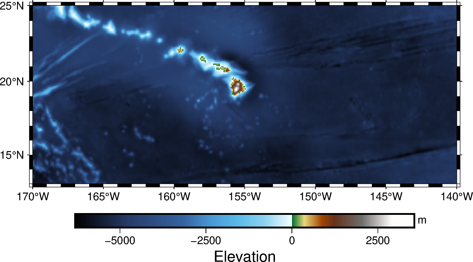
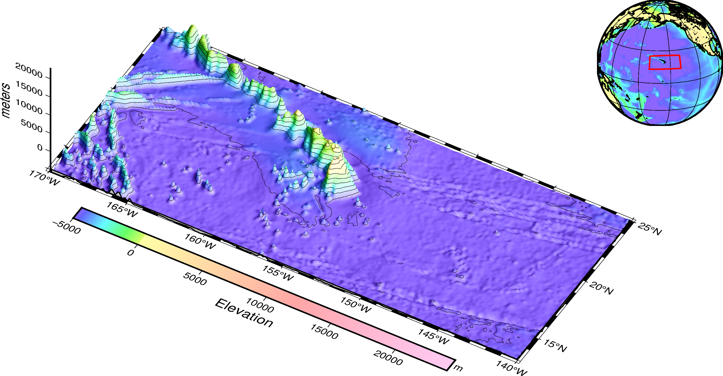
When we read about Olympus Mons, it is usually compared to Everest here on Earth. However, the most interesting thing is to compare it with another mountain range taking as a reference the abyssal seabed (without the ocean) - Hawaii. Interestingly, in terms of latitudes and longitudes on the planet, these two features are in almost the same position. To match the approximate dimensions, let’s crop a sample of the Earth Global Relief using pygmt.datasets with slices of 12 degrees of latitude and 30 degrees of longitude.

# get SRTM around Hawaii 
topo_hawaii = pygmt.datasets.load_earth_relief(region=[-170,-140,13,25],resolution="05m")

# and get the whole Earth at the same resolution of our low resolution Mars dataset
topo_globe = pygmt.datasets.load_earth_relief(region=[-180,180,-90,90],resolution="01d")

And we use the same sequence as above to make a map.

# second things, second

fig = pygmt.Figure()
# note I can add projection, after cmap and after, frame (and control frame)
fig.grdimage(grid=topo_hawaii,projection='M12c',frame='a5f1',cmap='geo')
# also, I can add a colorbar (later)
fig.colorbar(frame=["a2500", "x+lElevation", "y+lm"])

fig.show()

Another few notes

As we want to make a comparison, let’s keep the same color scale as Mars, still using as a basis for the Z plane, -5000 meters (see the line plane="-5000+ggrey" exactly like the map above. The inset in the upper right corner is the same and we adjust the bounding box coordinates used to cut out the topography, drawing in red on the map.

fig = pygmt.Figure()
# note I can add projection, after cmap and after, frame (and control frame)
frame =  ["xa5f1","ya5f1", "z5000+lmeters", "wSEnZ"]

topo_cpt = pygmt.makecpt(cmap='sealand',series=f'-5000/24000/1000',continuous=True)

fig.grdview(grid=topo_hawaii,
            region=[-170,-140,13,25,-5000,23000],
            frame=frame,
            perspective=[150,45],
            projection='M15c',
            zsize='4c',
            surftype='s',
            cmap=topo_cpt,
            plane="-5000+ggrey",
            shading='+a100+nt1',
            # Set the contour pen thickness to "0.1p"
            contourpen="0.1p",)

fig.colorbar(perspective=True, frame=["a5000", "x+lElevation", "y+lm"])

bounds = [[-170.,13.],
          [-170.,25.],
          [-140.,25.],
          [-140.,13.],
          [-170.,13.]]

with fig.inset(position="JTR+w3.5c+o0.2c", margin=0, box=None):
    # Create a figure in the inset using the global projection centered at Olympus MOns
    fig.grdimage(grid=topo_globe,region='g',frame='g',projection='G-160/19/3.5c"')
    fig.coast(region='g',shorelines="thin", frame="g")
    fig.plot(bounds,pen="1p,red")
    
fig.show()

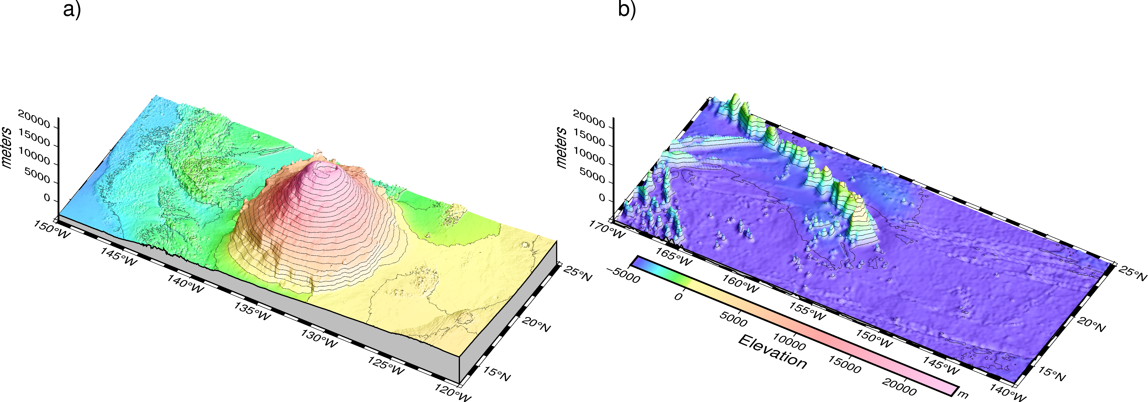
Combining the two maps side by side¶

Basically it’s the same blocks as above, just using pygmt’s Figure.set_panel mechanism to tile.

fig = pygmt.Figure()

with fig.subplot(
    nrows=1, ncols=2, figsize=("28c", "16c"), autolabel=True, margins="1c"
):
    with fig.set_panel(panel=0):

        topo_cpt = pygmt.makecpt(cmap='sealand',series=f'-5000/24000/1000',continuous=True)

        frame =  ["xa5f1","ya5f1", "z5000+lmeters", "wSEnZ"]

        fig.grdview(grid=dset_olympus,
                    region=[210,240,13,25,-5000,23000],
                    frame=frame,
                    perspective=[150,45],
                    projection='M',
                    zsize='4c',
                    surftype='s',
                    cmap=topo_cpt,
                    plane="-5000+ggrey",
                    shading='+a100+nt1',
                    # Set the contour pen thickness to "0.1p"
                    contourpen="0.1p",)

        # we don't need the colormap in both figures
        #fig.colorbar(perspective=True, frame=["a5000", "x+lElevation", "y+lm"])
        
    with fig.set_panel(panel=1):
        frame =  ["xa5f1","ya5f1", "z5000+lmeters", "wSEnZ"]

        topo_cpt = pygmt.makecpt(cmap='sealand',series=f'-5000/24000/1000',continuous=True)

        fig.grdview(grid=topo_hawaii,
                    region=[-170,-140,13,25,-5000,23000],
                    frame=frame,
                    perspective=[150,45],
                    projection='M',
                    zsize='4c',
                    surftype='s',
                    cmap=topo_cpt,
                    plane="-5000+ggrey",
                    shading='+a100+nt1',
                    # Set the contour pen thickness to "0.1p"
                    contourpen="0.1p",)

        fig.colorbar(perspective=True, frame=["a5000", "x+lElevation", "y+lm"])       

fig.show()

Bonus map¶

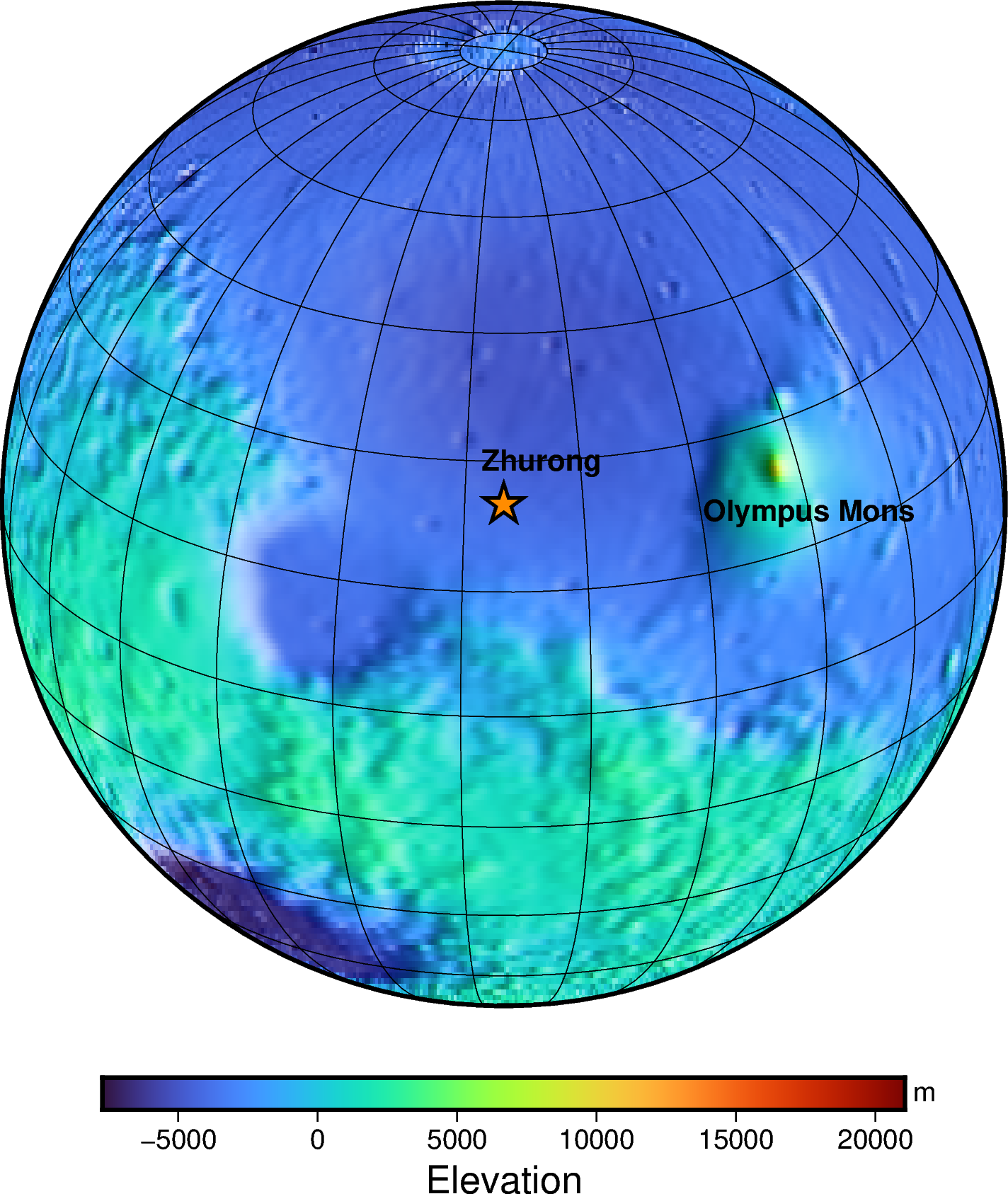
Recently the rover Zhurong from the Tianwen-1’s mission landed successfully at 109.926°E, 25.066°N, in southern Utopia Planitia on Mars (check out the article of Ye, B., Qian, Y., Xiao, L., Michalski, J. R., Li, Y., Wu, B., & Qiao, L. (2021). Geomorphologic exploration targets at the Zhurong landing site in the southern Utopia Planitia of Mars. Earth and Planetary Science Letters, 576, 117199. https://doi.org/10.1016/j.epsl.2021.117199). We can create a map of the region with the landing point.

First, let’s locate Utopia Planitia. Take a look at Figure 1 by Ye et al. (2021).

fig = pygmt.Figure()

# we are using a Orthographic view centered at the landing site
fig.grdimage(grid=dset_mars_topo,region='g',frame='g',projection='G109.926/25.066/12c"',shading='+a100+nt1')

zhurong = [109.926,25.066]
Olympus = [360-210,19.0] #position for Olympus Mons - see the letf border of the area

# and we drop a "star" in the landing site and write with a small displacement of text
fig.plot(x=zhurong[0],y=zhurong[1],style="a0.5c", pen="1p,black", color="darkorange")
fig.text(x=zhurong[0]+5,y=zhurong[1]+5, text="Zhurong", font='10p,Helvetica-Bold')

fig.text(x=Olympus[0],y=Olympus[1], text="Olympus Mons", font='10p,Helvetica-Bold')

fig.colorbar(frame=["a5000", "x+lElevation", "y+lm"])
fig.show()

Crafting beautiful maps with PyGMT

Making some Mars maps with pygmt (extended)

Contents