Tutorial 3 - scientific Python ecosystem 🐍: Xarray (gridded data 🌐)

In this tutorial we will to process and visualize raster data using PyGMT’s integration with Xarray.

Note

This tutorial is part of the AGU24 annual meeting GMT/PyGMT pre-conference workshop (PREWS9) Mastering Geospatial Visualizations with GMT/PyGMT

• Website: https://www.generic-mapping-tools.org/agu24workshop

• GitHub: GenericMappingTools/agu24workshop

• Conference: https://agu.confex.com/agu/agu24/meetingapp.cgi/Session/226736

History

• Author: Max Jones

• Created: November-December 2024

• Recommended versions: PyGMT v0.13.0 with GMT 6.5.0

Fee free to play around with these code examples 🚀. In case you found any kind of error, just report it by opening an issue or provide a fix via a pull request. Please use the GMT forum to ask questions.

0️⃣ What is Xarray?

Xarray is an open source project and Python package for working with n-dimensional data using labeled dimensions and coordinates.

1️⃣ Why use Xarray with PyGMT

Xarray provides a set of useful features for working with multi-dimensional data and unlocks even more functionality through its rich ecosystem. Some specific benefits of integrating Xarray and PyGMT include:

• Simplifying the extension of PyGMT functionality to 3-D+ datasets

• Access additional datasets, such as those located on the cloud

• Use out-of-core computing with libraries like Dask

• Interactively visualize by using Xarray, PyGMT, and dashboarding tools like Panel and Bokeh

• Work with both raster and vector data in memory

2️⃣ Getting started

First we’ll import all the libraries used throughout the tutorial.

import gcsfs
import pygmt
import xarray as xr

Let’s use a PyGMT function to explore an Xarray DataArray. We can use the pygmt.datasets.load_earth_relief function to load one of GMT’s remote datasets. This will take longer the first time that it’s run because GMT downloads the data from the GMT server. We’ll specify the server in order to quicken download speeds to Washington, D.C., USA.

with pygmt.config(GMT_DATA_SERVER="NOAA"):
    grid = pygmt.datasets.load_earth_relief(resolution="01d")
grid

gmtread [NOTICE]: Remote data courtesy of GMT data server NOAA [http://noaa.generic-mapping-tools.org]

gmtread [NOTICE]: SRTM15 Earth Relief v2.6 at 1x1 arc degrees reduced by Gaussian Cartesian filtering (314.5 km fullwidth) [Tozer et al., 2019].

gmtread [NOTICE]:   -> Download grid file [112K]: earth_relief_01d_g.grd

<xarray.DataArray 'z' (lat: 181, lon: 361)> Size: 523kB
array([[ 2865. ,  2865. ,  2865. , ...,  2865. ,  2865. ,  2865. ],
       [ 3088. ,  3087.5,  3087. , ...,  3088.5,  3088. ,  3088. ],
       [ 3100.5,  3100.5,  3101. , ...,  3101.5,  3101. ,  3100.5],
       ...,
       [-3745.5, -3731. , -3723. , ..., -3734. , -3741.5, -3745.5],
       [-2939.5, -2945. , -2950.5, ..., -2895. , -2921. , -2939.5],
       [-3861. , -3861. , -3861. , ..., -3861. , -3861. , -3861. ]])
Coordinates:
  * lat      (lat) float64 1kB -90.0 -89.0 -88.0 -87.0 ... 87.0 88.0 89.0 90.0
  * lon      (lon) float64 3kB -180.0 -179.0 -178.0 -177.0 ... 178.0 179.0 180.0
Attributes:
    Conventions:       CF-1.7
    title:             SRTM15 Earth Relief v2.6 at 01 arc degree
    history:           
    description:       IGPP Earth relief
    long_name:         elevation (m)
    units:             meters
    vertical_datum:    EGM96
    horizontal_datum:  WGS84

xarray.DataArray

'z'

• lat: 181
• lon: 361

• 2.865e+03 2.865e+03 2.865e+03 ... -3.861e+03 -3.861e+03 -3.861e+03

  array([[ 2865. ,  2865. ,  2865. , ...,  2865. ,  2865. ,  2865. ],
         [ 3088. ,  3087.5,  3087. , ...,  3088.5,  3088. ,  3088. ],
         [ 3100.5,  3100.5,  3101. , ...,  3101.5,  3101. ,  3100.5],
         ...,
         [-3745.5, -3731. , -3723. , ..., -3734. , -3741.5, -3745.5],
         [-2939.5, -2945. , -2950.5, ..., -2895. , -2921. , -2939.5],
         [-3861. , -3861. , -3861. , ..., -3861. , -3861. , -3861. ]])

• Coordinates: (2)
  • lat
    (lat)
    float64
    -90.0 -89.0 -88.0 ... 89.0 90.0

    long_name :

    latitude

    units :

    degrees_north

    standard_name :

    latitude

    axis :

    Y

    array([-90., -89., -88., -87., -86., -85., -84., -83., -82., -81., -80., -79.,
           -78., -77., -76., -75., -74., -73., -72., -71., -70., -69., -68., -67.,
           -66., -65., -64., -63., -62., -61., -60., -59., -58., -57., -56., -55.,
           -54., -53., -52., -51., -50., -49., -48., -47., -46., -45., -44., -43.,
           -42., -41., -40., -39., -38., -37., -36., -35., -34., -33., -32., -31.,
           -30., -29., -28., -27., -26., -25., -24., -23., -22., -21., -20., -19.,
           -18., -17., -16., -15., -14., -13., -12., -11., -10.,  -9.,  -8.,  -7.,
            -6.,  -5.,  -4.,  -3.,  -2.,  -1.,   0.,   1.,   2.,   3.,   4.,   5.,
             6.,   7.,   8.,   9.,  10.,  11.,  12.,  13.,  14.,  15.,  16.,  17.,
            18.,  19.,  20.,  21.,  22.,  23.,  24.,  25.,  26.,  27.,  28.,  29.,
            30.,  31.,  32.,  33.,  34.,  35.,  36.,  37.,  38.,  39.,  40.,  41.,
            42.,  43.,  44.,  45.,  46.,  47.,  48.,  49.,  50.,  51.,  52.,  53.,
            54.,  55.,  56.,  57.,  58.,  59.,  60.,  61.,  62.,  63.,  64.,  65.,
            66.,  67.,  68.,  69.,  70.,  71.,  72.,  73.,  74.,  75.,  76.,  77.,
            78.,  79.,  80.,  81.,  82.,  83.,  84.,  85.,  86.,  87.,  88.,  89.,
            90.])

  • lon
    (lon)
    float64
    -180.0 -179.0 ... 179.0 180.0

    long_name :

    longitude

    units :

    degrees_east

    standard_name :

    longitude

    axis :

    X

    array([-180., -179., -178., ...,  178.,  179.,  180.])

• Indexes: (2)
  • lat
    PandasIndex

    PandasIndex(Index([-90.0, -89.0, -88.0, -87.0, -86.0, -85.0, -84.0, -83.0, -82.0, -81.0,
           ...
            81.0,  82.0,  83.0,  84.0,  85.0,  86.0,  87.0,  88.0,  89.0,  90.0],
          dtype='float64', name='lat', length=181))

  • lon
    PandasIndex

    PandasIndex(Index([-180.0, -179.0, -178.0, -177.0, -176.0, -175.0, -174.0, -173.0, -172.0,
           -171.0,
           ...
            171.0,  172.0,  173.0,  174.0,  175.0,  176.0,  177.0,  178.0,  179.0,
            180.0],
          dtype='float64', name='lon', length=361))

• Attributes: (8)

  Conventions :

  CF-1.7

  title :

  SRTM15 Earth Relief v2.6 at 01 arc degree

  history :

  description :

  IGPP Earth relief

  long_name :

  elevation (m)

  units :

  meters

  vertical_datum :

  EGM96

  horizontal_datum :

  WGS84

3️⃣ Plotting raster data

We can pass this dataset to Figure.grdimage to plot the dataset, specifying a projection and colormap. We use the Winkel Tripel projection (“R”) with a 12c width to show the whole world.

fig = pygmt.Figure()
fig.grdimage(grid=grid, projection="R12c", cmap="SCM/oleron", frame=True)
fig.show()

4️⃣ Processing raster data

All of the PyGMT raster processing functions can accept and return Xarray DataArrays. As one example, we’ll use the grdgradient function to create a hillshade raster. This will calculate the reflection of a light source projecting from west to east at an altitude of 30 degrees.

region = [-119.825, -119.4, 37.6, 37.825]
grid = pygmt.datasets.load_earth_relief(resolution="03s", region=region)

hillshade = pygmt.grdgradient(grid=grid, radiance=[270, 30])
hillshade

grdblend [NOTICE]: Remote data courtesy of GMT data server oceania [http://oceania.generic-mapping-tools.org]

grdblend [NOTICE]: Earth Relief at 3x3 arc seconds tiles provided by SRTMGL3 (land only) [NASA/USGS].

grdblend [NOTICE]:   -> Download 1x1 degree grid tile (earth_relief_03s_g): N37W120

<xarray.DataArray 'z' (lat: 271, lon: 511)> Size: 1MB
array([[-0.30839247, -0.37808514, -0.30799666, ...,  0.12039052,
         0.20474193, -0.17929687],
       [-0.09469072, -0.3017121 , -0.31324536, ...,  0.0442035 ,
         0.06209851, -0.07466871],
       [-0.95000005, -0.95000005, -0.26423818, ...,  0.04321925,
         0.03116445,  0.13370842],
       ...,
       [-0.44154865, -0.31297821, -0.20481637, ..., -0.1700097 ,
        -0.22448991, -0.25389677],
       [-0.74398577, -0.27561006, -0.31929246, ..., -0.1227859 ,
        -0.1983598 , -0.20921303],
       [-0.42644808, -0.35136998, -0.39577812, ..., -0.04772562,
        -0.19724692, -0.21158722]])
Coordinates:
  * lat      (lat) float64 2kB 37.6 37.6 37.6 37.6 ... 37.82 37.82 37.82 37.83
  * lon      (lon) float64 4kB -119.8 -119.8 -119.8 ... -119.4 -119.4 -119.4
Attributes:
    Conventions:   CF-1.7
    title:         Produced by grdgradient
    history:       gmt grdgradient @GMTAPI@-S-I-G-M-G-N-000000 -E270/30 -G@GM...
    description:   Lambertian radiance
    long_name:     z
    actual_range:  [ 508. 3533.]

xarray.DataArray

'z'

• lat: 271
• lon: 511

• -0.3084 -0.3781 -0.308 -0.3086 ... 0.0546 -0.04773 -0.1972 -0.2116

  array([[-0.30839247, -0.37808514, -0.30799666, ...,  0.12039052,
           0.20474193, -0.17929687],
         [-0.09469072, -0.3017121 , -0.31324536, ...,  0.0442035 ,
           0.06209851, -0.07466871],
         [-0.95000005, -0.95000005, -0.26423818, ...,  0.04321925,
           0.03116445,  0.13370842],
         ...,
         [-0.44154865, -0.31297821, -0.20481637, ..., -0.1700097 ,
          -0.22448991, -0.25389677],
         [-0.74398577, -0.27561006, -0.31929246, ..., -0.1227859 ,
          -0.1983598 , -0.20921303],
         [-0.42644808, -0.35136998, -0.39577812, ..., -0.04772562,
          -0.19724692, -0.21158722]])

• Coordinates: (2)
  • lat
    (lat)
    float64
    37.6 37.6 37.6 ... 37.82 37.83

    long_name :

    latitude

    units :

    degrees_north

    standard_name :

    latitude

    axis :

    Y

    actual_range :

    [37.6 37.825]

    array([37.6     , 37.600833, 37.601667, ..., 37.823333, 37.824167, 37.825   ])

  • lon
    (lon)
    float64
    -119.8 -119.8 ... -119.4 -119.4

    long_name :

    longitude

    units :

    degrees_east

    standard_name :

    longitude

    axis :

    X

    actual_range :

    [-119.825 -119.4 ]

    array([-119.825   , -119.824167, -119.823333, ..., -119.401667, -119.400833,
           -119.4     ])

• Indexes: (2)
  • lat
    PandasIndex

    PandasIndex(Index([ 37.59999999999999,  37.60083333333332,  37.60166666666665,
           37.602499999999985,  37.60333333333332,  37.60416666666666,
            37.60499999999999,  37.60583333333332, 37.606666666666655,
            37.60749999999999,
           ...
                      37.8175, 37.818333333333335,  37.81916666666667,
                        37.82,  37.82083333333333,  37.82166666666667,
           37.822500000000005,  37.82333333333334,  37.82416666666667,
                       37.825],
          dtype='float64', name='lat', length=271))

  • lon
    PandasIndex

    PandasIndex(Index([           -119.825, -119.82416666666667, -119.82333333333334,
                     -119.8225, -119.82166666666667, -119.82083333333334,
           -119.82000000000001, -119.81916666666667, -119.81833333333334,
           -119.81750000000001,
           ...
                     -119.4075, -119.40666666666667, -119.40583333333333,
                      -119.405, -119.40416666666667, -119.40333333333334,
                     -119.4025, -119.40166666666667, -119.40083333333334,
                        -119.4],
          dtype='float64', name='lon', length=511))

• Attributes: (6)

  Conventions :

  CF-1.7

  title :

  Produced by grdgradient

  history :

  gmt grdgradient @GMTAPI@-S-I-G-M-G-N-000000 -E270/30 -G@GMTAPI@-S-O-G-G-G-Y-000001

  description :

  Lambertian radiance

  long_name :

  z

  actual_range :

  [ 508. 3533.]

Let’s plot the result using the same grdimage function shared earlier, this time using a custom colormap.

fig = pygmt.Figure()
pygmt.makecpt(cmap="SCM/grayC", series=[-1.5, 0.3, 0.01])
fig.grdimage(
    grid=hillshade,
    projection="M12c",
    frame=["lSEt", "xa0.1", "ya0.1"],
    cmap=True,
)
fig

5️⃣ Download data and load with Xarray

Most times you’ll want to use your own data rather than the sample datasets. Here we show how to use the which functionality to download a NetCDF file available via https.

# Download the dataset from the IRI Data Library
url = "https://iridl.ldeo.columbia.edu/SOURCES/.NOAA/.NODC/.WOA09/.Grid-1x1/.Annual/.temperature/.t_an/data.nc"
netcdf_file = pygmt.which(fname=url, download=True)
woa_temp = xr.open_dataset(netcdf_file).isel(time=0)
woa_temp

<xarray.Dataset> Size: 9MB
Dimensions:  (depth: 33, lat: 180, lon: 360)
Coordinates:
  * depth    (depth) float32 132B 0.0 10.0 20.0 30.0 ... 4.5e+03 5e+03 5.5e+03
  * lat      (lat) float32 720B -89.5 -88.5 -87.5 -86.5 ... 86.5 87.5 88.5 89.5
  * lon      (lon) float32 1kB 0.5 1.5 2.5 3.5 4.5 ... 356.5 357.5 358.5 359.5
    time     datetime64[ns] 8B 2008-01-01
Data variables: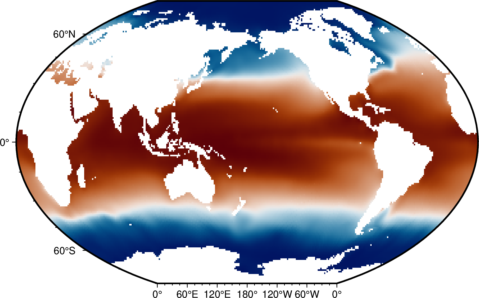
    t_an     (depth, lat, lon) float32 9MB ...

xarray.Dataset

• Dimensions:
  • depth: 33
  • lat: 180
  • lon: 360
• Coordinates: (4)
  • depth
    (depth)
    float32
    0.0 10.0 20.0 ... 5e+03 5.5e+03

    positive :

    down

    description :

    Standard Depth Levels

    axis :

    Z

    standard_name :

    depth

    long_name :

    depth

    gridtype :

    0

    units :

    m

    array([   0.,   10.,   20.,   30.,   50.,   75.,  100.,  125.,  150.,  200.,
            250.,  300.,  400.,  500.,  600.,  700.,  800.,  900., 1000., 1100.,
           1200., 1300., 1400., 1500., 1750., 2000., 2500., 3000., 3500., 4000.,
           4500., 5000., 5500.], dtype=float32)

  • lat
    (lat)
    float32
    -89.5 -88.5 -87.5 ... 88.5 89.5

    pointwidth :

    1.0

    axis :

    Y

    description :

    Latitude Range: -90 to 90 degrees with 0 at the Equator and increasing along the north.

    standard_name :

    latitude

    long_name :

    latitude

    bounds :

    lat_bnds

    gridtype :

    0

    units :

    degree_north

    array([-89.5, -88.5, -87.5, -86.5, -85.5, -84.5, -83.5, -82.5, -81.5, -80.5,
           -79.5, -78.5, -77.5, -76.5, -75.5, -74.5, -73.5, -72.5, -71.5, -70.5,
           -69.5, -68.5, -67.5, -66.5, -65.5, -64.5, -63.5, -62.5, -61.5, -60.5,
           -59.5, -58.5, -57.5, -56.5, -55.5, -54.5, -53.5, -52.5, -51.5, -50.5,
           -49.5, -48.5, -47.5, -46.5, -45.5, -44.5, -43.5, -42.5, -41.5, -40.5,
           -39.5, -38.5, -37.5, -36.5, -35.5, -34.5, -33.5, -32.5, -31.5, -30.5,
           -29.5, -28.5, -27.5, -26.5, -25.5, -24.5, -23.5, -22.5, -21.5, -20.5,
           -19.5, -18.5, -17.5, -16.5, -15.5, -14.5, -13.5, -12.5, -11.5, -10.5,
            -9.5,  -8.5,  -7.5,  -6.5,  -5.5,  -4.5,  -3.5,  -2.5,  -1.5,  -0.5,
             0.5,   1.5,   2.5,   3.5,   4.5,   5.5,   6.5,   7.5,   8.5,   9.5,
            10.5,  11.5,  12.5,  13.5,  14.5,  15.5,  16.5,  17.5,  18.5,  19.5,
            20.5,  21.5,  22.5,  23.5,  24.5,  25.5,  26.5,  27.5,  28.5,  29.5,
            30.5,  31.5,  32.5,  33.5,  34.5,  35.5,  36.5,  37.5,  38.5,  39.5,
            40.5,  41.5,  42.5,  43.5,  44.5,  45.5,  46.5,  47.5,  48.5,  49.5,
            50.5,  51.5,  52.5,  53.5,  54.5,  55.5,  56.5,  57.5,  58.5,  59.5,
            60.5,  61.5,  62.5,  63.5,  64.5,  65.5,  66.5,  67.5,  68.5,  69.5,
            70.5,  71.5,  72.5,  73.5,  74.5,  75.5,  76.5,  77.5,  78.5,  79.5,
            80.5,  81.5,  82.5,  83.5,  84.5,  85.5,  86.5,  87.5,  88.5,  89.5],
          dtype=float32)

  • lon
    (lon)
    float32
    0.5 1.5 2.5 ... 357.5 358.5 359.5

    pointwidth :

    1.0

    modulus :

    360.0

    axis :

    X

    description :

    Longitude Range: 0 to 360 degrees with 0 at Greenwich Meridian and increasing along the east.

    standard_name :

    longitude

    long_name :

    longitude

    bounds :

    lon_bnds

    gridtype :

    1

    units :

    degree_east

    array([  0.5,   1.5,   2.5, ..., 357.5, 358.5, 359.5], dtype=float32)

  • time
    ()
    datetime64[ns]
    2008-01-01

    pointwidth :

    0

    gridtype :

    0

    array('2008-01-01T00:00:00.000000000', dtype='datetime64[ns]')

• Data variables: (1)
  • t_an
    (depth, lat, lon)
    float32
    ...

    cell_methods :

    time:mean within years time:mean over years

    grid_mapping :

    crs

    standard_name :

    sea_water_temperature

    long_name :

    Sea Water Temperature

    units :

    degrees Celsius

    description :

    The objectively interpolated mean field for Sea Water Temperature for annual time period at each one-degree square at each standard depth.

    [2138400 values with dtype=float32]

• Indexes: (3)
  • depth
    PandasIndex

    PandasIndex(Index([   0.0,   10.0,   20.0,   30.0,   50.0,   75.0,  100.0,  125.0,  150.0,
            200.0,  250.0,  300.0,  400.0,  500.0,  600.0,  700.0,  800.0,  900.0,
           1000.0, 1100.0, 1200.0, 1300.0, 1400.0, 1500.0, 1750.0, 2000.0, 2500.0,
           3000.0, 3500.0, 4000.0, 4500.0, 5000.0, 5500.0],
          dtype='float32', name='depth'))

  • lat
    PandasIndex

    PandasIndex(Index([-89.5, -88.5, -87.5, -86.5, -85.5, -84.5, -83.5, -82.5, -81.5, -80.5,
           ...
            80.5,  81.5,  82.5,  83.5,  84.5,  85.5,  86.5,  87.5,  88.5,  89.5],
          dtype='float32', name='lat', length=180))

  • lon
    PandasIndex

    PandasIndex(Index([  0.5,   1.5,   2.5,   3.5,   4.5,   5.5,   6.5,   7.5,   8.5,   9.5,
           ...
           350.5, 351.5, 352.5, 353.5, 354.5, 355.5, 356.5, 357.5, 358.5, 359.5],
          dtype='float32', name='lon', length=360))

• Attributes: (0)

# Make a static plot of sea surface temperature
fig = pygmt.Figure()
fig.grdimage(grid=woa_temp.t_an.sel(depth=0), cmap="vik", projection="R15c", frame=True)
fig.show()

grdinfo [WARNING]: No 3-D array in file /home/runner/work/agu24workshop/agu24workshop/book/data.nc.  Selecting first 3-D slice in the 4-D array t_an

6️⃣ Open data directly from the cloud

Xarray allows you to open data directly from cloud object storage. This can be useful to avoid downloading the entire dataset, since Xarray can subset to a specific section of interest before loading the data into memory.

Here we show this functionality based on Xarray’s tutorial. We’ll load a specific dataset from the Coupled Model Intercomparison Project Phase 6 (CMIP6), calculate the sea level change between 2015 and 2100, and plot the results using PyGMT.

First, let’s load CMIP6 data from Google Cloud Storage

fs = gcsfs.GCSFileSystem(token="anon")

store = fs.get_mapper(
    "gs://cmip6/CMIP6/ScenarioMIP/NOAA-GFDL/GFDL-ESM4/ssp585/r1i1p1f1/Omon/zos/gr/v20180701/"
)
ds = xr.open_zarr(store=store, consolidated=True)
ds

<xarray.Dataset> Size: 268MB
Dimensions:    (lat: 180, bnds: 2, lon: 360, time: 1032)
Coordinates:
  * lat        (lat) float64 1kB -89.5 -88.5 -87.5 -86.5 ... 86.5 87.5 88.5 89.5
    lat_bnds   (lat, bnds) float64 3kB ...
  * lon        (lon) float64 3kB 0.5 1.5 2.5 3.5 4.5 ... 356.5 357.5 358.5 359.5
    lon_bnds   (lon, bnds) float64 6kB ...
  * time       (time) object 8kB 2015-01-16 12:00:00 ... 2100-12-16 12:00:00
    time_bnds  (time, bnds) object 17kB ...
Dimensions without coordinates: bnds
Data variables:
    zos        (time, lat, lon) float32 267MB ...
Attributes: (12/49)
    Conventions:            CF-1.7 CMIP-6.0 UGRID-1.0
    activity_id:            ScenarioMIP
    branch_method:          standard
    branch_time_in_child:   60225.0
    branch_time_in_parent:  60225.0
    comment:                <null ref>
    ...                     ...
    tracking_id:            hdl:21.14100/21c772eb-064e-4c75-8e16-da95bbfd29b7...
    variable_id:            zos
    variant_info:           N/A
    variant_label:          r1i1p1f1
    netcdf_tracking_ids:    hdl:21.14100/21c772eb-064e-4c75-8e16-da95bbfd29b7...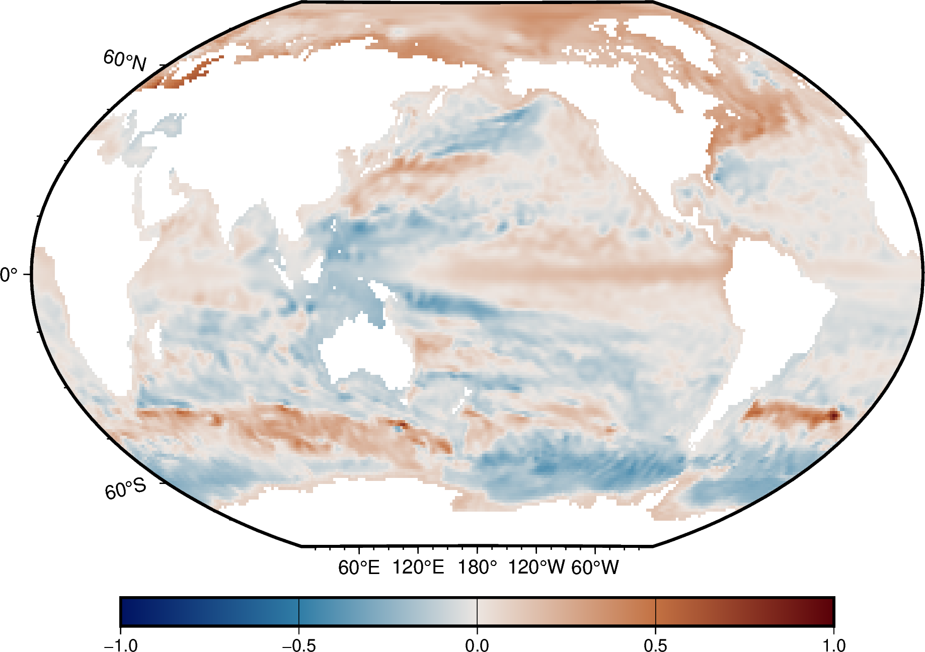
    version_id:             v20180701

xarray.Dataset

• Dimensions:
  • lat: 180
  • bnds: 2
  • lon: 360
  • time: 1032
• Coordinates: (6)
  • lat
    (lat)
    float64
    -89.5 -88.5 -87.5 ... 88.5 89.5

    axis :

    Y

    bounds :

    lat_bnds

    cell_methods :

    time: point

    long_name :

    latitude

    standard_name :

    latitude

    units :

    degrees_north

    array([-89.5, -88.5, -87.5, -86.5, -85.5, -84.5, -83.5, -82.5, -81.5, -80.5,
           -79.5, -78.5, -77.5, -76.5, -75.5, -74.5, -73.5, -72.5, -71.5, -70.5,
           -69.5, -68.5, -67.5, -66.5, -65.5, -64.5, -63.5, -62.5, -61.5, -60.5,
           -59.5, -58.5, -57.5, -56.5, -55.5, -54.5, -53.5, -52.5, -51.5, -50.5,
           -49.5, -48.5, -47.5, -46.5, -45.5, -44.5, -43.5, -42.5, -41.5, -40.5,
           -39.5, -38.5, -37.5, -36.5, -35.5, -34.5, -33.5, -32.5, -31.5, -30.5,
           -29.5, -28.5, -27.5, -26.5, -25.5, -24.5, -23.5, -22.5, -21.5, -20.5,
           -19.5, -18.5, -17.5, -16.5, -15.5, -14.5, -13.5, -12.5, -11.5, -10.5,
            -9.5,  -8.5,  -7.5,  -6.5,  -5.5,  -4.5,  -3.5,  -2.5,  -1.5,  -0.5,
             0.5,   1.5,   2.5,   3.5,   4.5,   5.5,   6.5,   7.5,   8.5,   9.5,
            10.5,  11.5,  12.5,  13.5,  14.5,  15.5,  16.5,  17.5,  18.5,  19.5,
            20.5,  21.5,  22.5,  23.5,  24.5,  25.5,  26.5,  27.5,  28.5,  29.5,
            30.5,  31.5,  32.5,  33.5,  34.5,  35.5,  36.5,  37.5,  38.5,  39.5,
            40.5,  41.5,  42.5,  43.5,  44.5,  45.5,  46.5,  47.5,  48.5,  49.5,
            50.5,  51.5,  52.5,  53.5,  54.5,  55.5,  56.5,  57.5,  58.5,  59.5,
            60.5,  61.5,  62.5,  63.5,  64.5,  65.5,  66.5,  67.5,  68.5,  69.5,
            70.5,  71.5,  72.5,  73.5,  74.5,  75.5,  76.5,  77.5,  78.5,  79.5,
            80.5,  81.5,  82.5,  83.5,  84.5,  85.5,  86.5,  87.5,  88.5,  89.5])

  • lat_bnds
    (lat, bnds)
    float64
    ...

    axis :

    Y

    long_name :

    latitude bounds

    units :

    degrees_north

    [360 values with dtype=float64]

  • lon
    (lon)
    float64
    0.5 1.5 2.5 ... 357.5 358.5 359.5

    axis :

    X

    bounds :

    lon_bnds

    cell_methods :

    time: point

    long_name :

    longitude

    standard_name :

    longitude

    units :

    degrees_east

    array([  0.5,   1.5,   2.5, ..., 357.5, 358.5, 359.5])

  • lon_bnds
    (lon, bnds)
    float64
    ...

    axis :

    X

    long_name :

    longitude bounds

    units :

    degrees_east

    [720 values with dtype=float64]

  • time
    (time)
    object
    2015-01-16 12:00:00 ... 2100-12-...

    axis :

    T

    bounds :

    time_bnds

    calendar_type :

    noleap

    description :

    Temporal mean

    long_name :

    time

    standard_name :

    time

    array([cftime.DatetimeNoLeap(2015, 1, 16, 12, 0, 0, 0, has_year_zero=True),
           cftime.DatetimeNoLeap(2015, 2, 15, 0, 0, 0, 0, has_year_zero=True),
           cftime.DatetimeNoLeap(2015, 3, 16, 12, 0, 0, 0, has_year_zero=True),
           ...,
           cftime.DatetimeNoLeap(2100, 10, 16, 12, 0, 0, 0, has_year_zero=True),
           cftime.DatetimeNoLeap(2100, 11, 16, 0, 0, 0, 0, has_year_zero=True),
           cftime.DatetimeNoLeap(2100, 12, 16, 12, 0, 0, 0, has_year_zero=True)],
          dtype=object)

  • time_bnds
    (time, bnds)
    object
    ...

    long_name :

    time axis boundaries

    [2064 values with dtype=object]

• Data variables: (1)
  • zos
    (time, lat, lon)
    float32
    ...

    cell_measures :

    area: areacello

    cell_methods :

    area: mean where sea time: mean

    comment :

    Model data on the 1x1 grid includes values in all cells for which any ocean exists on the native grid. For mapping purposes, we recommend using a land mask such as World Ocean Atlas to cover these areas of partial land. For calculating approximate integrals, we recommend multiplying by cell area (areacello).

    interp_method :

    conserve_order1

    long_name :

    Sea Surface Height Above Geoid

    original_name :

    zos

    standard_name :

    sea_surface_height_above_geoid

    units :

    m

    [66873600 values with dtype=float32]

• Indexes: (3)
  • lat
    PandasIndex

    PandasIndex(Index([-89.5, -88.5, -87.5, -86.5, -85.5, -84.5, -83.5, -82.5, -81.5, -80.5,
           ...
            80.5,  81.5,  82.5,  83.5,  84.5,  85.5,  86.5,  87.5,  88.5,  89.5],
          dtype='float64', name='lat', length=180))

  • lon
    PandasIndex

    PandasIndex(Index([               0.5, 1.5000000000000002,                2.5,
                          3.5,                4.5,                5.5,
                          6.5,  7.499999999999999,                8.5,
                          9.5,
           ...
           350.50000000000006,              351.5,              352.5,
                        353.5,              354.5,              355.5,
                        356.5,              357.5,              358.5,
           359.50000000000006],
          dtype='float64', name='lon', length=360))

  • time
    PandasIndex

    PandasIndex(CFTimeIndex([2015-01-16 12:00:00, 2015-02-15 00:00:00, 2015-03-16 12:00:00,
                 2015-04-16 00:00:00, 2015-05-16 12:00:00, 2015-06-16 00:00:00,
                 2015-07-16 12:00:00, 2015-08-16 12:00:00, 2015-09-16 00:00:00,
                 2015-10-16 12:00:00,
                 ...
                 2100-03-16 12:00:00, 2100-04-16 00:00:00, 2100-05-16 12:00:00,
                 2100-06-16 00:00:00, 2100-07-16 12:00:00, 2100-08-16 12:00:00,
                 2100-09-16 00:00:00, 2100-10-16 12:00:00, 2100-11-16 00:00:00,
                 2100-12-16 12:00:00],
                dtype='object', length=1032, calendar='noleap', freq=None))

• Attributes: (49)

  Conventions :

  CF-1.7 CMIP-6.0 UGRID-1.0

  activity_id :

  ScenarioMIP

  branch_method :

  standard

  branch_time_in_child :

  60225.0

  branch_time_in_parent :

  60225.0

  comment :

  <null ref>

  contact :

  gfdl.climate.model.info@noaa.gov

  creation_date :

  2019-06-18T16:38:22Z

  data_specs_version :

  01.00.27

  experiment :

  update of RCP8.5 based on SSP5

  experiment_id :

  ssp585

  external_variables :

  areacello

  forcing_index :

  1

  frequency :

  mon

  further_info_url :

  https://furtherinfo.es-doc.org/CMIP6.NOAA-GFDL.GFDL-ESM4.ssp585.none.r1i1p1f1

  grid :

  ocean data regridded from tripolar - nominal 0.5 deg latitude/longitude to 180,360; interpolation method: conserve_order1

  grid_label :

  gr

  history :

  File was processed by fremetar (GFDL analog of CMOR). TripleID: [exper_id_FlJGh4Wo6W,realiz_id_kt2pvOSbWt,run_id_1S546GMKbs]

  initialization_index :

  1

  institution :

  National Oceanic and Atmospheric Administration, Geophysical Fluid Dynamics Laboratory, Princeton, NJ 08540, USA

  institution_id :

  NOAA-GFDL

  license :

  CMIP6 model data produced by NOAA-GFDL is licensed under a Creative Commons Attribution-ShareAlike 4.0 International License (https://creativecommons.org/licenses/). Consult https://pcmdi.llnl.gov/CMIP6/TermsOfUse for terms of use governing CMIP6 output, including citation requirements and proper acknowledgment. Further information about this data, including some limitations, can be found via the further_info_url (recorded as a global attribute in this file). The data producers and data providers make no warranty, either express or implied, including, but not limited to, warranties of merchantability and fitness for a particular purpose. All liabilities arising from the supply of the information (including any liability arising in negligence) are excluded to the fullest extent permitted by law.

  mip_era :

  CMIP6

  nominal_resolution :

  1x1 degree

  parent_activity_id :

  CMIP

  parent_experiment_id :

  historical

  parent_mip_era :

  CMIP6

  parent_source_id :

  GFDL-ESM4

  parent_time_units :

  days since 1850-1-1

  parent_variant_label :

  r1i1p1f1

  physics_index :

  1

  product :

  model-output

  realization_index :

  1

  realm :

  ocean

  references :

  see further_info_url attribute

  source :

  GFDL-ESM4 (2018): atmos: GFDL-AM4.1 (Cubed-sphere (c96) - 1 degree nominal horizontal resolution; 360 x 180 longitude/latitude; 49 levels; top level 1 Pa) ocean: GFDL-OM4p5 (GFDL-MOM6, tripolar - nominal 0.5 deg; 720 x 576 longitude/latitude; 75 levels; top grid cell 0-2 m) seaIce: GFDL-SIM4p5 (GFDL-SIS2.0, tripolar - nominal 0.5 deg; 720 x 576 longitude/latitude; 5 layers; 5 thickness categories) land: GFDL-LM4.1 aerosol: interactive atmosChem: GFDL-ATMCHEM4.1 (full atmospheric chemistry) ocnBgchem: GFDL-COBALTv2 landIce: GFDL-LM4.1 (GFDL ID: 2019_0301)

  source_id :

  GFDL-ESM4

  source_type :

  AOGCM AER CHEM BGC

  status :

  2020-10-03;created; by gcs.cmip6.ldeo@gmail.com

  sub_experiment :

  none

  sub_experiment_id :

  none

  table_id :

  Omon

  title :

  NOAA GFDL GFDL-ESM4 model output prepared for CMIP6 update of RCP8.5 based on SSP5

  tracking_id :

  hdl:21.14100/21c772eb-064e-4c75-8e16-da95bbfd29b7 hdl:21.14100/52017fc2-111d-4537-8ee5-ce1c5cca69b5 hdl:21.14100/ca0140ef-576c-49bc-bdbc-5da3427142b0 hdl:21.14100/207a8ede-0637-411b-866e-d18c5ff2e7f0 hdl:21.14100/59af902a-5b2e-445e-9af3-13383dd882d2

  variable_id :

  zos

  variant_info :

  N/A

  variant_label :

  r1i1p1f1

  netcdf_tracking_ids :

  hdl:21.14100/21c772eb-064e-4c75-8e16-da95bbfd29b7 hdl:21.14100/52017fc2-111d-4537-8ee5-ce1c5cca69b5 hdl:21.14100/ca0140ef-576c-49bc-bdbc-5da3427142b0 hdl:21.14100/207a8ede-0637-411b-866e-d18c5ff2e7f0 hdl:21.14100/59af902a-5b2e-445e-9af3-13383dd882d2

  version_id :

  v20180701

Calculate the different in sea level between a date in 2100 and 2015

zos_2015jan = ds.zos.sel(time="2015-01-16").squeeze()
zos_2100dec = ds.zos.sel(time="2100-12-16").squeeze()
sealevelchange = zos_2100dec - zos_2015jan

Make a plot of the difference in sea level

fig = pygmt.Figure()
pygmt.makecpt(cmap="vik", series=[-1, 1, 0.5], continuous=True)
fig.grdimage(grid=sealevelchange, cmap=True, projection="R15c", frame=True)
fig.colorbar()
fig.show()