Spectral indices with Landsat 8 imagery
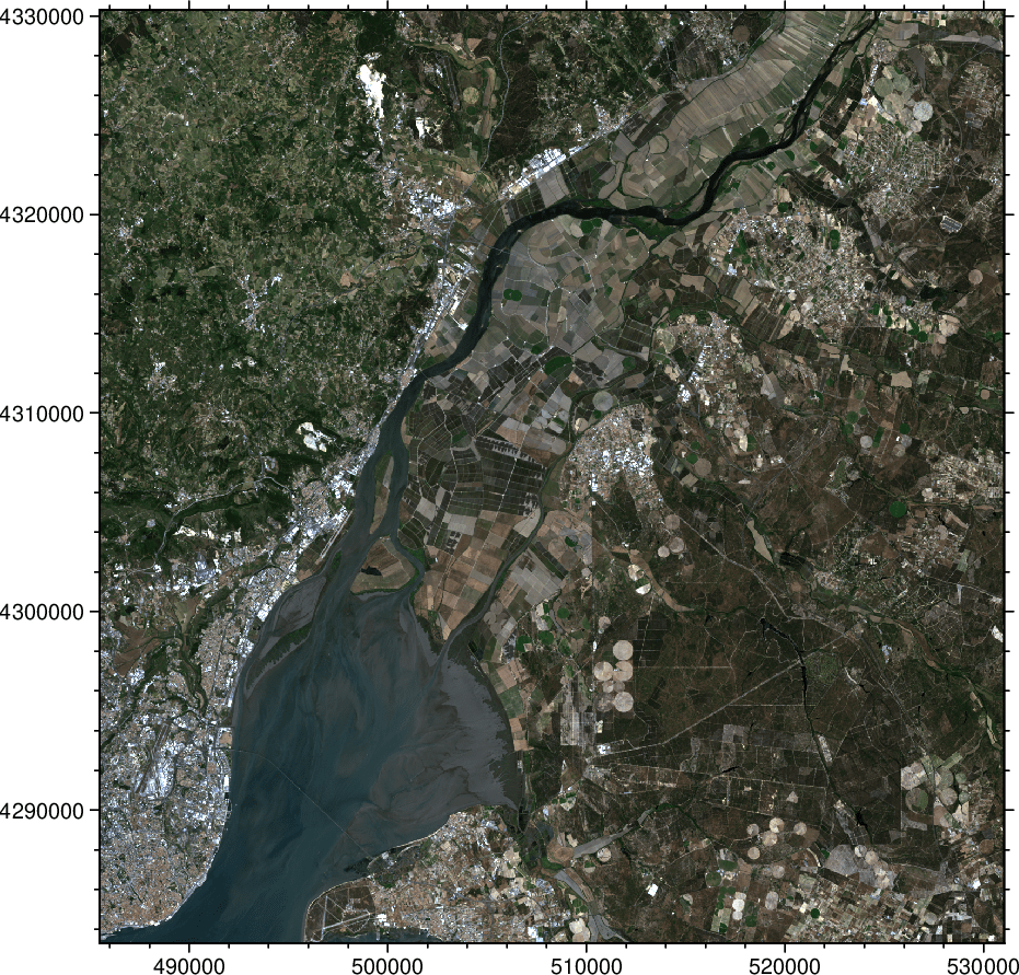
We will use here the same data cube that was introduced in the images example.
A very popular spectral indice is the NDVI which is deffined as the a normalized difference between the Near Infra Red (NIR) and the Red bands. Namely NDVI = (NIR - Red) / (NIR + Red). An heuristic says that NDVI values ~greater than 0.4 indicate green vegetation as higher the indice (maximum = 1) larger is the green vegetation content.
Since the data cube holds in it the information about each band, computing the NDVI is a trivial opration because we known where each band is in the data cube. Let's see it.
using RemoteS, GMT
N = ndvi("LC08_L1TP_20210525_02_cube.tiff");
imshow(N, colorbar=true)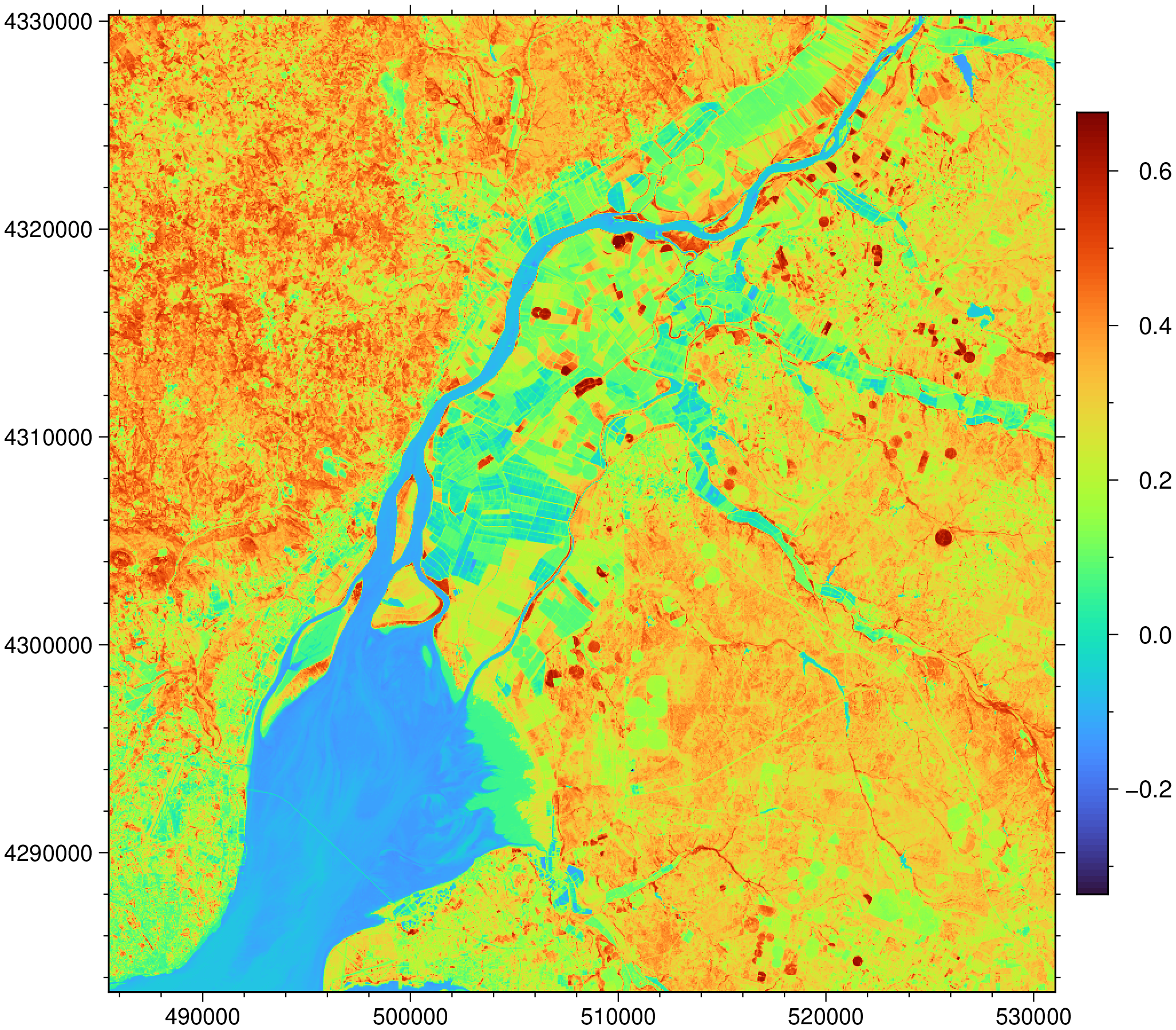
The spectral indices functions all have a $threshold$ value that will NaNify all values $< threshold$. Below we wipe out all values < 0.4 to show only the Green stuff
N = ndvi("LC08_L1TP_20210525_02_cube.tiff", threshold=0.4);
imshow(N, dpi=150, colorbar=1)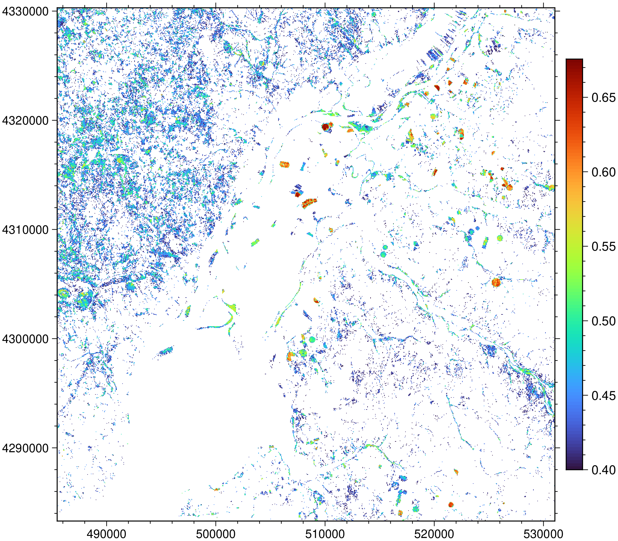
Cool but I would like to check that the result is correct.
The spectral indices functions have another option to obtain just a mask where the values are $> threshold$, so we can use it to mask out the true color image and see what we get.
# Compute a mask based on the condition that threshold >= 0.4
mask = ndvi("LC08_L1TP_20210525_02_cube.tiff", threshold=0.4, mask=true);
To mask out the true color image the best way is to use the mask as the alpha band. To make it easier we will recalculate the true color image here.
# Recalculate the true color image
Irgb = truecolor("LC08_L1TP_20210525_02_cube.tiff");

# Apply the mask
image_alpha!(Irgb, alpha_band=mask, burn=1);

# And save it to disk
gmtwrite("rgb_masked.tiff", Irgb)

imshow(Irgb)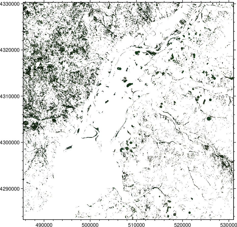
While we can see that only the green color is present in the above image, it's not easy to see the details. So let's zoom in but do also another thing. Let us see also what parts of the RGB image were not selected. To see that we will calculate the $inverse mask$, that is, the mask that retains all values < threshold. To achieve that we use the $mask$ option with a negative number.
# Compute a mask based on the condition that threshold >= 0.4
mask_inv = ndvi("LC08_L1TP_20210525_02_cube.tiff", threshold=0.4, mask=-1)
;
# Recompute the true color image that was modified by the ``image_alpha!`` step above
Irgb = truecolor("LC08_L1TP_20210525_02_cube.tiff");

image_alpha!(Irgb, alpha_band=mask_inv, burn=1);
gmtwrite("rgb_inv_masked.tiff", Irgb)
Plot the green vegetation that passed the NDVI threshold test and the other part, side by side.
grdimage("rgb_masked.tiff", region=(502380,514200,4311630,4321420), figsize=8, frame=:bare)
grdimage!("rgb_inv_masked.tiff", figsize=8, projection=:linear, xshift=8, frame=:bare, show=true)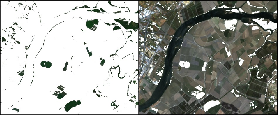
As we can see only the greenest part, the one that is probably more irrigated considering that all the river and cannals margins were retained, was extracted with the condition NDVI > 0.4. Off course, using different threshold values would lead to slightly different results.