Getting Started with Cloud-Native HLS Data in Julia:
Extracting an EVI Time Series from Harmonized Landsat-8 Sentinel-2 (HLS) data in the Cloud using CMR's SpatioTemporal Asset Catalog (CMR-STAC). This tutorial demonstrates how to work with the HLS Landsat 8 (HLSL30.015) and Sentinel-2 (HLSS30.015) data products.
NOTE: This tutorial is adapted from Getting Started with Cloud-Native HLS Data in Python
1. Importing packages
using HTTP, JSON, GMT, RemoteS

r = HTTP.request("GET", "https://cmr.earthdata.nasa.gov/stac/");
stac_response = JSON.parse(String(r.body));
2. Navigating the CMR-STAC API
What is STAC?
STAC is a specification that provides a common language for interpreting geospatial information in order to standardize indexing and discovering data.
Four STAC Specifications:
STAC Catalog: Contains a JSON file of links that organize all of the collections available.
Search for LP DAAC Catalogs, and print the information contained in the Catalog that we will be using today, LPCLOUD
stac_lp = [s for s in stac_response["links"] if occursin("LP", s["title"])]

# LPCLOUD is the STAC catalog we will be using and exploring today
hr = [s for s in stac_lp if s["title"] == "LPCLOUD"][1]["href"];
r = HTTP.request("GET", hr);
lp_cloud = JSON.parse(String(r.body));
Print the links contained in the LP CLOUD STAC Catalog
lp_links = lp_cloud["links"];

for l in lp_links
    try
        println(l["href"], " is the ", l["title"])
    catch
        println(l["href"])
    end
end
https://cmr.earthdata.nasa.gov/stac/LPCLOUD is the Provider catalog
https://cmr.earthdata.nasa.gov/stac/ is the Root catalog
https://cmr.earthdata.nasa.gov/stac/LPCLOUD/collections is the Provider Collections
https://cmr.earthdata.nasa.gov/stac/LPCLOUD/search is the Provider Item Search
https://cmr.earthdata.nasa.gov/stac/LPCLOUD/search is the Provider Item Search
https://cmr.earthdata.nasa.gov/stac/LPCLOUD/conformance is the Conformance Classes
https://api.stacspec.org/v1.0.0-beta.1/openapi.yaml is the OpenAPI Doc
https://api.stacspec.org/v1.0.0-beta.1/index.html is the HTML documentation
https://cmr.earthdata.nasa.gov/stac/LPCLOUD/collections/ASTGTM.v003
https://cmr.earthdata.nasa.gov/stac/LPCLOUD/collections/HLSL30.v2.0
https://cmr.earthdata.nasa.gov/stac/LPCLOUD/collections/HLSL30.v1.5
https://cmr.earthdata.nasa.gov/stac/LPCLOUD/collections/HLSS30.v1.5
https://cmr.earthdata.nasa.gov/stac/LPCLOUD/collections/HLSS30.v2.03. STAC Collection: Extension of STAC Catalog containing additional information that describe the STAC Items in that Collection.
Get a response from the LPCLOUD Collection and print the information included in the response.
# Set collections endpoint to variable
lp_collections = [l["href"] for l in lp_links if l["rel"] == "collections"][1];

# Call collections endpoint
r = HTTP.request("GET", lp_collections);
collections_response = JSON.parse(String(r.body));

println("This collection contains $(collections_response["description"]) ($(length(collections_response["collections"])) available)")
This collection contains All collections provided by LPCLOUD (5 available)As of October 3, 2021, there are five collections available, and more will be added in the future.
Print out one of the collections:
collections = collections_response["collections"];
collections[2]
Dict{String, Any} with 8 entries:
"links" => Any[Dict{String, Any}("rel"=>"self", "href"=>"https://cmr.e…
"id" => "HLSL30.v2.0"
"stac_version" => "1.0.0"
"title" => "HLS Landsat Operational Land Imager Surface Reflectance an…
"license" => "not-provided"
"type" => "Collection"
"description" => "The Harmonized Landsat and Sentinel-2 (HLS) project provid…
"extent" => Dict{String, Any}("spatial"=>Dict{String, Any}("bbox"=>Any[…In CMR, id is used to query by a specific product, so be sure to save the ID for the HLS S30 and L30 V1.5 products below:
# Search available collections for HLS and print them out
hls_collections = [c for c in collections if contains(c["title"], "HLS")];

[println("$(h["title"]) has ID (shortname) of: $(h["id"])") for h in hls_collections]
HLS Landsat Operational Land Imager Surface Reflectance and TOA Brightness Daily Global 30m v2.0 has ID (shortname) of: HLSL30.v2.0
HLS Operational Land Imager Surface Reflectance and TOA Brightness Daily Global 30 m V1.5 has ID (shortname) of: HLSL30.v1.5
HLS Sentinel-2 Multi-spectral Instrument Surface Reflectance Daily Global 30 m V1.5 has ID (shortname) of: HLSS30.v1.5
HLS Sentinel-2 Multi-spectral Instrument Surface Reflectance Daily Global 30m v2.0 has ID (shortname) of: HLSS30.v2.0
4-element Vector{Nothing}:
nothing
nothing
nothing
nothingNote that the
idshortname is in the format: productshortname.vVVV (where VVV = product version)
Explore the attributes contained in the HLSS30 Collection.
# Grab HLSS30 collection
s30 = [h for h in hls_collections if h["id"] == "HLSS30.v1.5"][1];

# Check out the extent of this collection
for k in keys(s30["extent"]) println(k, " : ", s30["extent"][k]) end
spatial : Dict{String, Any}("bbox" => Any[Any[-180, -90, 180, 90]])
temporal : Dict{String, Any}("interval" => Any[Any["2015-12-01T00:00:00.000Z", nothing]])So here we can see that the extent is global, and can also see the temporal range–where None means on-going or to present.
println("HLS S30 Start Date is: $(s30["extent"]["temporal"]["interval"][1][1])")HLS S30 Start Date is: 2015-12-01T00:00:00.000ZNext, explore the attributes of the HLSL30 collection.
Above, notice that the L30 product has a different start date than the S30 product.
4. STAC Item: Represents data and metadata assets that are spatiotemporally coincident
Query the HLSS30 collection for items and return the first item in the collection.
# Go through all links in the collection and return the link containing the items endpoint

# Set items endpoint to variable
s30_items = [s["href"] for s in s30["links"] if s["rel"] == "items"][1]"https://cmr.earthdata.nasa.gov/stac/LPCLOUD/collections/HLSS30.v1.5/items"# Call items endpoint
r = HTTP.request("GET", s30_items);
s30_items_response = JSON.parse(String(r.body));
s30_item = s30_items_response["features"][1]Dict{String, Any} with 10 entries:
"links" => Any[Dict{String, Any}("rel"=>"self", "href"=>"https://cm…
"stac_extensions" => Any["https://stac-extensions.github.io/eo/v1.0.0/schema.…
"geometry" => Dict{String, Any}("coordinates"=>Any[Any[Any[40.9215, 19…
"id" => "HLS.S30.T37QGC.2016228T074942.v1.5"
"stac_version" => "1.0.0"
"properties" => Dict{String, Any}("datetime"=>"2016-08-15T08:00:59.720Z"…
"bbox" => Any[40.9089, 19.7977, 41.1665, 20.7895]
"type" => "Feature"
"assets" => Dict{String, Any}("B8A"=>Dict{String, Any}("href"=>"http…
"collection" => "HLSS30.v1.5"STAC metadata provides valuable information on the item, including a unique ID, when it was acquired, the location of the observation, and a cloud cover assessment.
# Print metadata attributes from this observation
println("The ID for this item is: $(s30_item["id"])")
println("It was acquired on: $(s30_item["properties"]["datetime"]))")
println("over: $(s30_item["bbox"]) (Lower Left, Upper Right corner coordinates)")
println("It contains $(length(s30_item["assets"])) assets")
println("and is $(s30_item["properties"]["eo:cloud_cover"])% cloudy.")
The ID for this item is: HLS.S30.T37QGC.2016228T074942.v1.5
It was acquired on: 2016-08-15T08:00:59.720Z)
over: Any[40.908869, 19.797714, 41.166492, 20.789487] (Lower Left, Upper Right corner coordinates)
It contains 20 assets
and is 4% cloudy.Print out the ten items and the percent cloud cover–we will use this to decidewhich item to visualize in the next section.
Using the information printed above, set the item_index below to whichever observation is the least cloudy above.
item_index = 2;

# Grab the next item in the list
s30_item = s30_items_response["features"][item_index];

println("The ID for this item is: $(s30_item["id"])")
println("It was acquired on: $(s30_item["properties"]["datetime"])")
println("over: $(s30_item["bbox"]) (Lower Left, Upper Right corner coordinates)")
println("It contains $(length(s30_item["assets"])) assets")
println("and is $(s30_item["properties"]["eo:cloud_cover"])% cloudy.")
The ID for this item is: HLS.S30.T37QEE.2016228T074942.v1.5
It was acquired on: 2016-08-15T08:00:59.720Z
over: Any[38.999805, 21.611674, 40.068079, 22.607038] (Lower Left, Upper Right corner coordinates)
It contains 20 assets
and is 0% cloudy.Print out the names of all of the assets included in this item.
println("The following assets are available for download:")
keys(s30_item["assets"])
The following assets are available for download:
KeySet for a Dict{String, Any} with 20 entries. Keys:
"B8A"
"SZA"
"B07"
"B05"
"B02"
"B06"
"B08"
"B01"
"B09"
"Fmask"
"VZA"
"B10"
"browse"
"B03"
"B04"
"VAA"
"metadata"
"SAA"
"B11"
"B12"Notice that each HLS item includes a browse image. Read the browse file into memory and visualize the HLS acquisition.
s30_item["assets"]["browse"]Dict{String, Any} with 3 entries:
"href" => "https://data.lpdaac.earthdatacloud.nasa.gov/lp-prod-public/HLSS30…
"title" => "Download HLS.S30.T37QEE.2016228T074942.v1.5.jpg"
"type" => "image/jpeg"img = gmtread(s30_item["assets"]["browse"]["href"]);
imshow(img)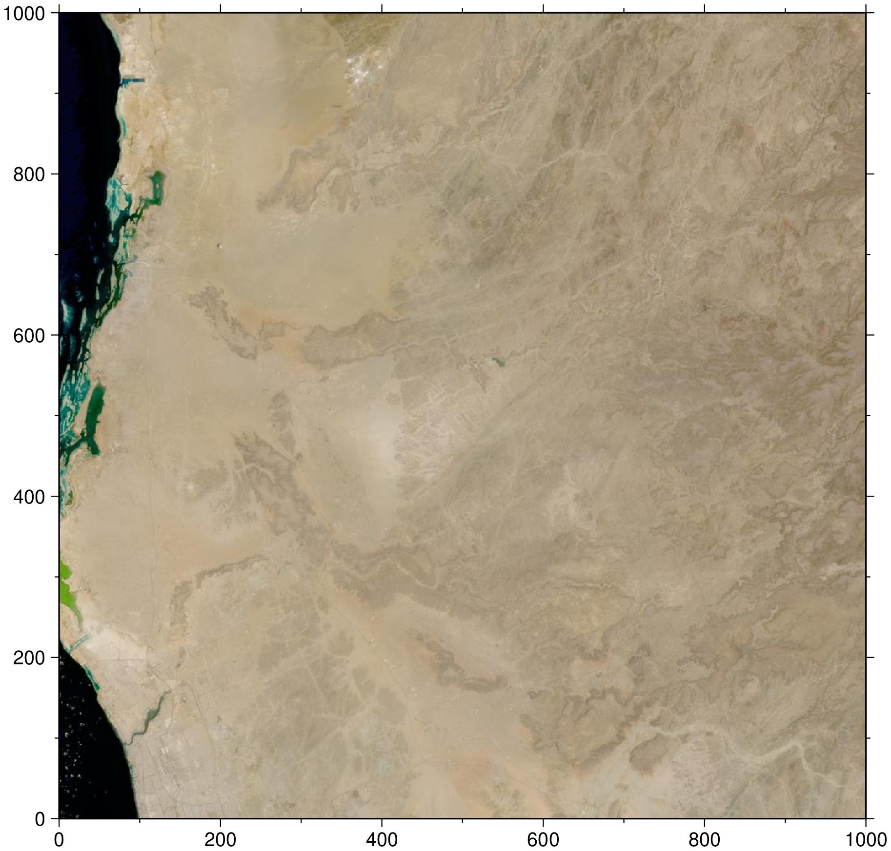
Congrats! You have pulled your first HLS asset from the cloud using STAC!
3. CMR-STAC API: Searching for Items
In this section, instead of simply navigating through the structure of a STAC Catalog, use the search endpoint to query the API by region of interest and time period of interest.
3.1 Spatial Querying via Bounding Box
The search endpoint is one of the links found in the LPCLOUD STAC Catalog, which can be leveraged to retrieve STAC Items that match the submitted query parameters.
Grab the search endpoint for the LPCLOUD STAC Catalog and send a POST request to retrieve items.
# Define the search endpoint
lp_search = [l["href"] for l in lp_links if l["rel"] == "search"][1]

# Set up a dictionary that will be used to POST requests to the search endpoint
params = Dict();
r = HTTP.request("POST", lp_search);
search_response = JSON.parse(String(r.body));
"$(length(search_response["features"])) items found""10 items found"If we just call the search endpoint directly, it will default to returning the first 10 granules. Below, set a limit to return the first 100 matching items. Additional information on the spec for adding parameters to a search query can be found at:
https://github.com/radiantearth/stac-api-spec/tree/master/item-search#query-parameters-and-fields.
# Add in a limit parameter to retrieve 100 items at a time.
lim = 100;
params["limit"] = lim;
Above, we have added the limit as a parameter to the dictionary that we will post to the search endpoint to submit our request for data. As we keep moving forward in the tutorial, we will continue adding parameters to the params dictionary.
# send POST request to retrieve first 100 items in the STAC collection
r = HTTP.post(lp_search, ["Content-Type" => "application/json"], JSON.json(params));
search_response = JSON.parse(String(r.body));

"$(length(search_response["features"])) items found"
"100 items found"Load in the spatial region of interest for our use case using GMT. You will need to have downloaded the Field_Boundary.geojson from the repo, and it must be stored in the current working directory in order to continue. If you are still encountering issues, you can add the entire filepath to the file (ex: D = gmtread(\"C:/Username/HLS-Tutorial/Field_Boundary.geojson\") and try again.
# Since the output is a vector of GMTdataset and all data is in first element
D = gdalread("c:/v/Field_Boundary.geojson")[1];
Plot the geometry of the farm field boundaries.
imshow(D, projection=:guess)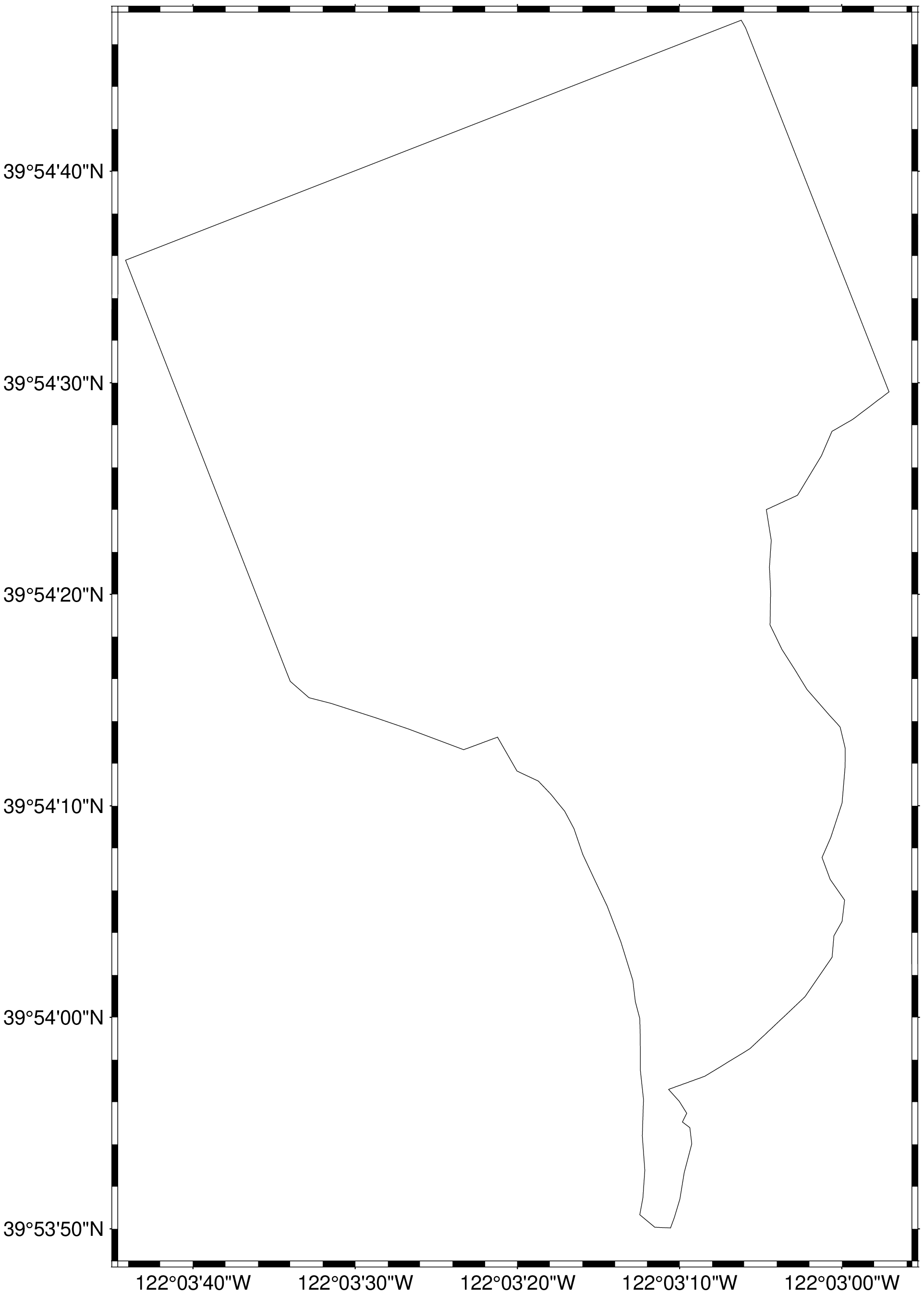
The farm field used in this example use case is located northwest of Chico, CA.
Now, add the bounding box of the region of interest to the CMR-STAC API Search query using the bbox parameter.
# Compute the polygon bounding cordinates
bb = gmtinfo(D, C=1)[1];

bbox = "$(bb[1]),$(bb[3]),$(bb[2]),$(bb[4])";
params["bbox"] = bbox;
paramsDict{Any, Any} with 2 entries:
"bbox" => "-122.0622682571411,39.897234301806,-122.04918980598451,39.9130938…
"limit" => 100# Send POST request with bbox included
r = HTTP.post(lp_search, ["Content-Type" => "application/json"], JSON.json(params));
search_response = JSON.parse(String(r.body));
"$(length(search_response["features"])) items found""100 items found"3.2 Temporal Querying
Finally, you can narrow your search to a specific time period of interest using the datetime parameter. Here we have set the time period of interest from September 2020 through March 2021. Additional information on setting temporal searches can be found in the NASA CMR Documentation.
# Define start time period / end time period
date_time = "2020-09-01T00:00:00Z/2021-03-31T23:59:59Z";

params["datetime"] = date_time
params
Dict{Any, Any} with 3 entries:
"datetime" => "2020-09-01T00:00:00Z/2021-03-31T23:59:59Z"
"bbox" => "-122.0622682571411,39.897234301806,-122.04918980598451,39.9130…
"limit" => 100# Send POST request with datetime included
r = HTTP.post(lp_search, ["Content-Type" => "application/json"], JSON.json(params))
search_response = JSON.parse(String(r.body));
"$(length(search_response["features"])) items found""100 items found"paramsDict{Any, Any} with 3 entries:
"datetime" => "2020-09-01T00:00:00Z/2021-03-31T23:59:59Z"
"bbox" => "-122.0622682571411,39.897234301806,-122.04918980598451,39.9130…
"limit" => 100As of October 4, 2021, the HLS Operational Land Imager Surface Reflectance and TOA Brightness (HLSL30) product has been provisionally released, and this tutorial has been updated to show how to combine observations from both products into a time series.
Next, add the shortname for the HLSS30 v1.5 product (HLSS30.v1.5) to the params dictionary, and query the CMR-STAC LPCLOUD search endpoint for just HLSS30 items.
s30_id = "HLSS30.v1.5"
params["collections"] = [s30_id];
# Search for the HLSS30 items of interest:
# Send POST request with collection included
r = HTTP.post(lp_search, ["Content-Type" => "application/json"], JSON.json(params))
s30_items = JSON.parse(String(r.body))["features"];
length(s30_items)61Append the HLSL30 V1.5 Product shortname (ID) to the list under the collections parameter.
l30_id = "HLSL30.v1.5";
append!(params["collections"], [l30_id])
params
Dict{Any, Any} with 4 entries:
"datetime" => "2020-09-01T00:00:00Z/2021-03-31T23:59:59Z"
"collections" => ["HLSS30.v1.5", "HLSL30.v1.5"]
"bbox" => "-122.0622682571411,39.897234301806,-122.04918980598451,39.9…
"limit" => 100The collections parameter is a list and can include multiple product collection short names.
# Search for the HLSS30 and HLSL30 items of interest:
# Send POST request with S30 and L30 collections included
r = HTTP.post(lp_search, ["Content-Type" => "application/json"], JSON.json(params))
hls_items = JSON.parse(String(r.body))["features"];
length(hls_items)684. Extracting HLS COGs from the Cloud
In this section, configure gdal and rasterio to use vsicurl to access the cloud assets that we are interested in, and read them directly into memory without needing to download the files.
# GDAL configurations used to successfully access LP DAAC Cloud Assets via vsicurl
set_config_option("GDAL_HTTP_COOKIEFILE", joinpath(tempdir(), "cookies.txt"))
set_config_option("GDAL_HTTP_COOKIEJAR", joinpath(tempdir(), "cookies.txt"))
set_config_option("GDAL_DISABLE_READDIR_ON_OPEN","YES")
set_config_option("CPL_VSIL_CURL_ALLOWED_EXTENSIONS","TIF")
set_config_option("CPL_VSIL_CURL_USE_HEAD","FALSE")
set_config_option("GDAL_HTTP_UNSAFESSL", "YES")
4.1 Subset by Band
View the contents of the first item.
h = hls_items[1]Dict{String, Any} with 10 entries:
"links" => Any[Dict{String, Any}("rel"=>"self", "href"=>"https://cm…
"stac_extensions" => Any["https://stac-extensions.github.io/eo/v1.0.0/schema.…
"geometry" => Dict{String, Any}("coordinates"=>Any[Any[Any[-121.964, 3…
"id" => "HLS.S30.T10TEK.2020273T190109.v1.5"
"stac_version" => "1.0.0"
"properties" => Dict{String, Any}("datetime"=>"2020-09-29T19:13:24.996Z"…
"bbox" => Any[-123.0, 39.657, -121.702, 40.6509]
"type" => "Feature"
"assets" => Dict{String, Any}("B8A"=>Dict{String, Any}("href"=>"http…
"collection" => "HLSS30.v1.5"Subset by band by filtering to only include the NIR, Red, Blue, and Quality (Fmask) layers in the list of links to access. Below you can find the different band numbers for each of the two products.
Sentinel 2:
evi_band_links = []

# Define which HLS product is being accessed
if (split(h["assets"]["browse"]["href"], '/')[5] == "HLSS30.015")
    evi_bands = ["B8A", "B04", "B02", "Fmask"] # NIR RED BLUE Quality for S30
else
    evi_bands = ["B05", "B04", "B02", "Fmask"] # NIR RED BLUE Quality for L30
end

# Subset the assets in the item down to only the desired bands
for a in h["assets"]
    for b in evi_bands
        if b == first(a)
            append!(evi_band_links, [h["assets"][first(a)]["href"]])
        end
    end
end

for e in evi_band_links  println(e)  end
https://lpdaac.earthdata.nasa.gov/lp-prod-protected/HLSS30.015/HLS.S30.T10TEK.2020273T190109.v1.5.B8A.tif
https://lpdaac.earthdata.nasa.gov/lp-prod-protected/HLSS30.015/HLS.S30.T10TEK.2020273T190109.v1.5.B02.tif
https://lpdaac.earthdata.nasa.gov/lp-prod-protected/HLSS30.015/HLS.S30.T10TEK.2020273T190109.v1.5.Fmask.tif
https://lpdaac.earthdata.nasa.gov/lp-prod-protected/HLSS30.015/HLS.S30.T10TEK.2020273T190109.v1.5.B04.tifRemember from above that you can always quickly load in the browse image to get a quick view of the item.
# Load jpg browse image into memory
image = gmtread(h["assets"]["browse"]["href"]);
imshow(image)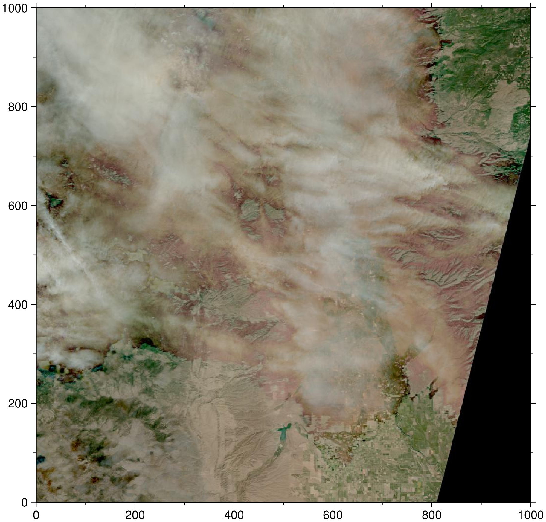
Above, we see a partly cloudy observation over the northern Central Valley of California.
4.2 Load a Spatially Subset HLS COG into Memory
Before loading the COGs into memory, run the cell below to check and make sure that you have a netrc file set up with your NASA Earthdata Login credentials, which will be needed to access the HLS files in the cells that follow. If you do not have a netrc file set up on your OS, the cell below should prompt you for your NASA Earthdata Login username and password.
set_config_option("GDAL_HTTP_COOKIEFILE", joinpath(tempdir(), "cookies.txt"));
set_config_option("GDAL_HTTP_COOKIEJAR", joinpath(tempdir(), "cookies.txt"));
set_config_option("GDAL_DISABLE_READDIR_ON_OPEN","YES");
set_config_option("CPL_VSIL_CURL_ALLOWED_EXTENSIONS","TIF");
set_config_option("CPL_VSIL_CURL_USE_HEAD","FALSE");
set_config_option("GDAL_HTTP_UNSAFESSL", "YES");
for e in evi_band_links
if split(e,'.')[end-1] == evi_bands[1] # NIR index
println("/vsicurl/"*e)
tic()
global nir = GMT.Gdal.read("/vsicurl/"*e)
toc()
elseif split(e,'.')[end-1] == evi_bands[2] # Red index
global red = GMT.Gdal.read("/vsicurl/"*e)
elseif split(e,'.')[end-1] == evi_bands[3] # Blue index
global blue = GMT.Gdal.read("/vsicurl/"*e)
elseif split(e,'.')[end-1] == evi_bands[4] # Mask index
global fmask = GMT.Gdal.read("/vsicurl/"*e)
end
end
println("The COGs have been loaded into memory!")/vsicurl/https://lpdaac.earthdata.nasa.gov/lp-prod-protected/HLSS30.015/HLS.S30.T10TEK.2020273T190109.v1.5.B8A.tif
elapsed time: 11.319765 seconds
The COGs have been loaded into memory!Getting an error in the section above? Accessing these files in the cloud requires you to authenticate using your NASA Earthdata Login account. You will need to have a netrc file set up containing those credentials in your home directory in order to successfully run the code
Below, take the farm field polygon and convert it from lat/lon (EPSG: 4326) into the native projection of HLS, UTM (aligned to the Military Grid Reference System). This must be done in order to use the Region of Interest (ROI) to subset the COG that is being pulled into memory–it must be in the native projection of the data being extracted.
utm = getproj(nir);        # Destination coordinate system
Dp  = lonlat2xy(D, utm);   # Project to UTM
Dp[1].geom = wkbPolygon;   # Ensure it's a polygon for the mask calculation
# Compute the projected polygon bounding cordinates
bb = gmtinfo(Dp, numeric=true)[1];Compute a mask with 1's inside the farm's polygon and 0's outside.
mask = gdalrasterize(Dp, ["-tr","30","30", "-te", "$(bb[1])", "$(bb[3])", "$(bb[2])", "$(bb[4])", "-burn", "1", "-init", "0"]);Now, we can use the ROI to mask any pixels that fall outside of it and crop to the bounding box. This greatly reduces the amount of data that are needed to load into memory.
nir_cropped = gdaltranslate(nir, ["-projwin", "$(bb[1])", "$(bb[4])", "$(bb[2])", "$(bb[3])"]);
red_cropped = gdaltranslate(red, ["-projwin", "$(bb[1])", "$(bb[4])", "$(bb[2])", "$(bb[3])"]);
blue_cropped = gdaltranslate(blue, ["-projwin", "$(bb[1])", "$(bb[4])", "$(bb[2])", "$(bb[3])"]);
fmask_cropped = gdaltranslate(fmask, ["-projwin", "$(bb[1])", "$(bb[4])", "$(bb[2])", "$(bb[3])"]);

@inbounds Threads.@threads for k = 1:length(fmask_cropped)
    (mask[k] == 0) && (fmask_cropped[k] = 1)
end
5. Processing HLS Data
In this section, read the file metadata to retrieve and apply the scale factor, filter out nodata values, define a function to calculate EVI, and execute the EVI function on the data loaded into memory. After that, perform quality filtering to screen out any poor quality observations.
Compute the EVI index using the evi function from the RemoreS package and plot the results.
EVI = evi(blue_cropped, red_cropped, nir_cropped);Apply a mask to the EVI layer using pixels with good quality as defined by the Fmask.
The good quality is encoded in the $fmask$ where its pixels are equal to zero.
# Replace the flagged values by NaN
@inbounds Threads.@threads for k = 1:length(EVI)
    (fmask_cropped[k] != 0) && (EVI[k] = NaN32)
end
# Display the EVI
imshow(EVI, colorbar=true)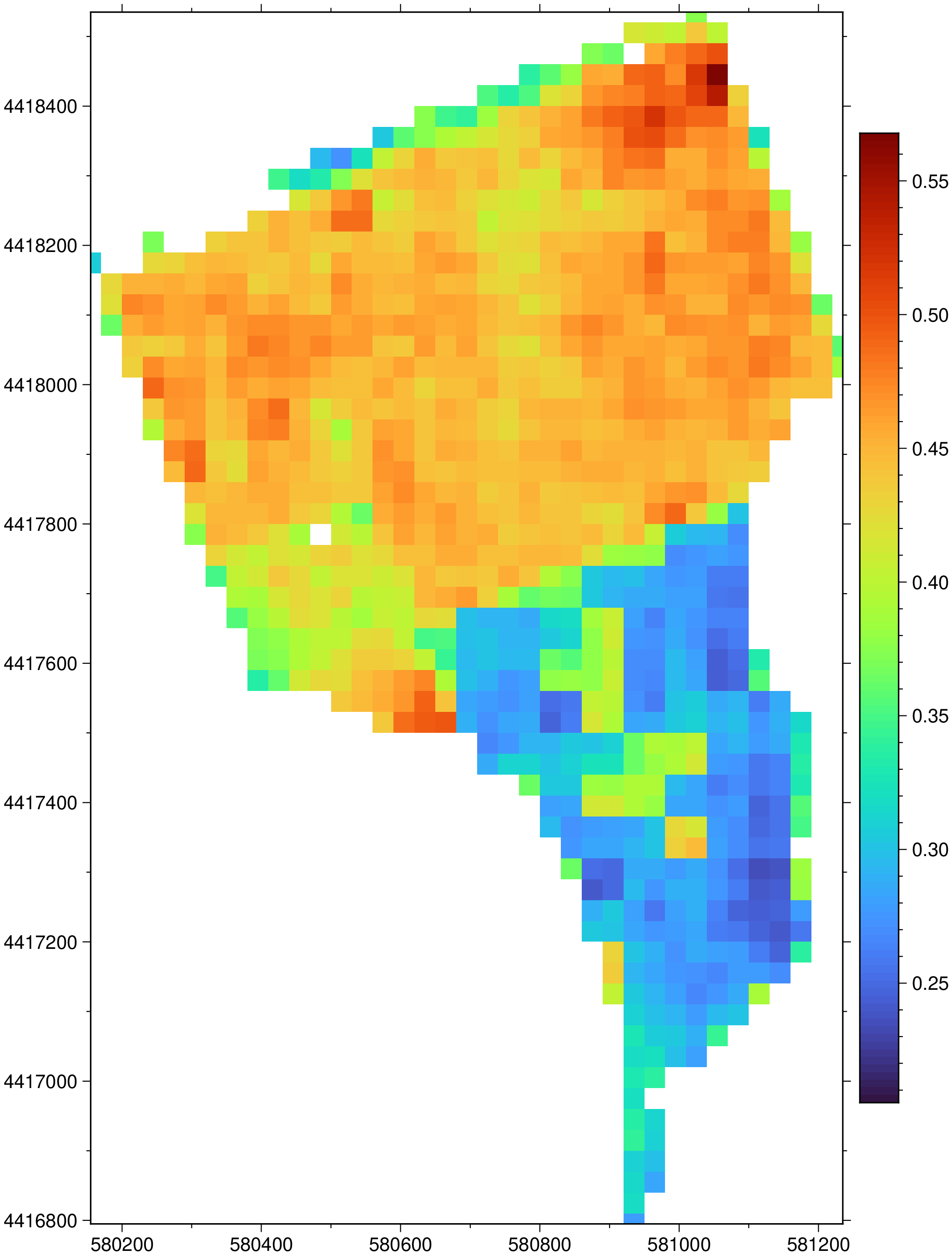
6. Automation
In this section, automate sections 4-5 for each HLS item that intersects our spatiotemporal subset of interest. Loop through each item and subset to the desired bands, load the spatial subset into memory, calculate EVI, quality filter, and save as a netCDF multi-layered cube.
Note: Be patient with the for loop below, it will take nearly an hour to complete.
# Put it all together and loop through each of the files, visualize, calculate statistics on EVI, and export
for (j, h) in enumerate(hls_items)

    outName = split(h["assets"]["browse"]["href"], '/')[end]
    outName = replace(outName, ".jpg" => "_EVI.grd")

    tic()
    try
        evi_band_links = []
        # Define which HLS product is being accessed
        if (split(h["assets"]["browse"]["href"], '/')[5] == "HLSS30.015")
            evi_bands = ["B8A", "B04", "B02", "Fmask"] # NIR RED BLUE Quality for S30
        else
            evi_bands = ["B05", "B04", "B02", "Fmask"] # NIR RED BLUE Quality for L30
        end

        for a in h["assets"]
            for b in evi_bands
                (b == first(a)) && append!(evi_band_links, [h["assets"][first(a)]["href"]])
            end
        end

        # Use vsicurl to load the data directly into memory (be patient, may take many seconds)
        for e in evi_band_links
            if split(e,'.')[end-1] == evi_bands[4] # Mask index
                local fmask = GMT.Gdal.read("/vsicurl/"*e);
                global fmask_cropped = gdaltranslate(fmask, ["-projwin", "$(bb[1])", "$(bb[4])", "$(bb[2])", "$(bb[3])"]);
                break
            end
        end

        @inbounds for k = 1:length(fmask_cropped)
            (mask[k] == 0) && (fmask_cropped[k] = 1)
        end

        all(fmask_cropped.image .!= 0) && continue

        for e in evi_band_links
            if split(e,'.')[end-1] == evi_bands[1] # NIR index
                global nir = GMT.Gdal.read("/vsicurl/"*e);
            elseif split(e,'.')[end-1] == evi_bands[2] # Red index
                global red = GMT.Gdal.read("/vsicurl/"*e);
            elseif split(e,'.')[end-1] == evi_bands[3] # Blue index
                global blue = GMT.Gdal.read("/vsicurl/"*e);
            end
        end

        nir_cropped = gdaltranslate(nir, ["-projwin", "$(bb[1])", "$(bb[4])", "$(bb[2])", "$(bb[3])"]);
        red_cropped = gdaltranslate(red, ["-projwin", "$(bb[1])", "$(bb[4])", "$(bb[2])", "$(bb[3])"]);
        blue_cropped = gdaltranslate(blue, ["-projwin", "$(bb[1])", "$(bb[4])", "$(bb[2])", "$(bb[3])"]);

        EVI = evi(blue_cropped, red_cropped, nir_cropped);

        # Replace the flagged values by NaN
        @inbounds for k = 1:length(EVI)
            (fmask_cropped[k] != 0) && (EVI[k] = NaN32)
        end

        #gmtwrite(outName, EVI)
        gdaltranslate(EVI, save=outName)
    catch err
        println(err)
    end
    toc()

    println("Processed file $j of $(length(hls_items))")
end
eviFiles = [o for o in readdir() if endswith(o, "EVI.grd")];df = dateformat"yyyymmddTHHMMSS";
time = Vector{TimeType}(undef, length(eviFiles));
for (i, e) in enumerate(eviFiles)
t = split(split(e, ".v1.5")[1], ".")[end];
# Julia doesn't parse a date in yyyyjjjT... so must resort to brewed functions
mon, day = monthday(doy2date(t[5:7], t[1:4]));
time[i] = DateTime(@sprintf("%s%.02d%.02d%s", t[1:4], mon, day, t[8:end]), df);
end
# Get the permutation vector p that puts time[p] in sorted order
p = sortperm(time);
eviFiles = eviFiles[p]; # Sort the file names in ascending time order
time = time[p]; # and the time too.Save all EVI estimations in a netCDF 3d (a cube) file
stackgrids(eviFiles, time, z_unit="unix", save="evi_cube.nc")Interpolate along all layers at a point with coordinates x = 580740; y = 4418042
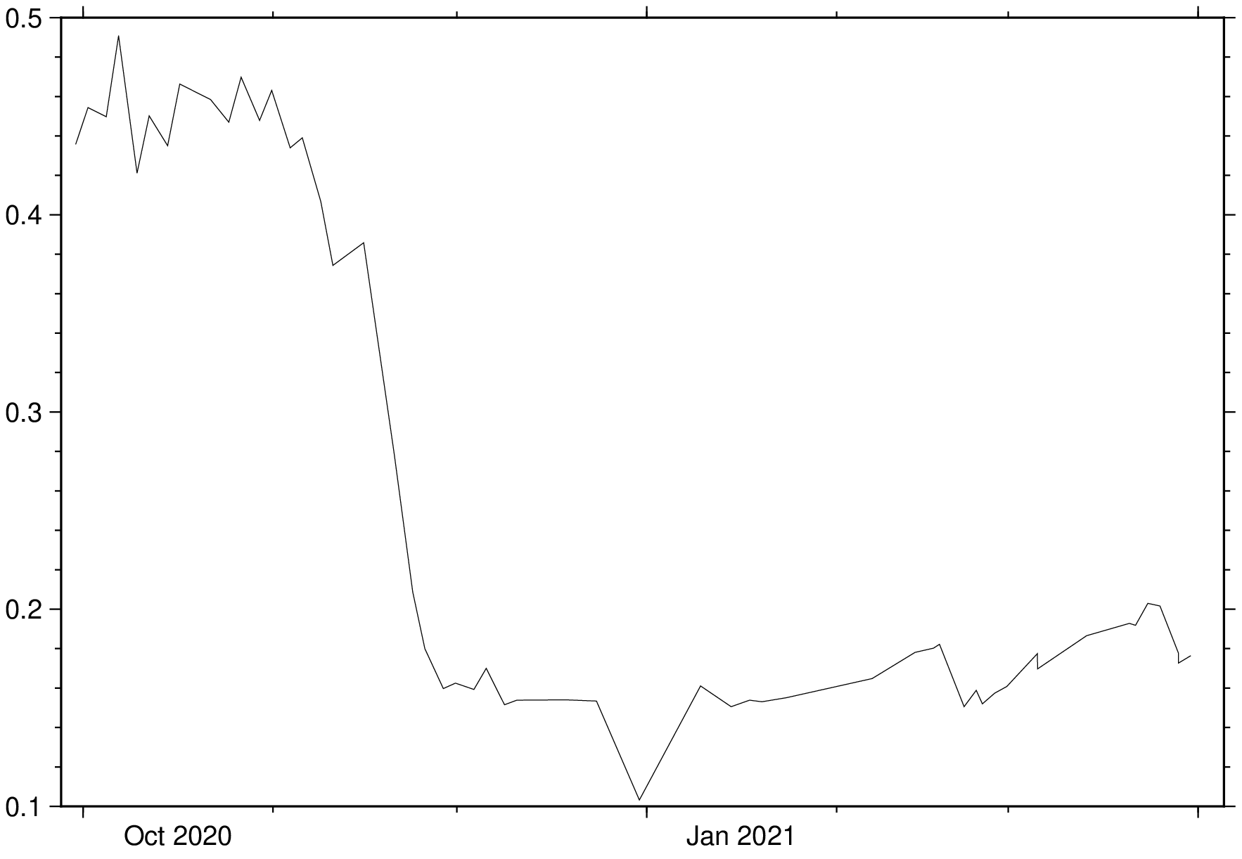
D = grdinterpolate("evi_cube.nc", pt=(580740,4418042));Now, plot the time series showing the distribution of EVI values for our farm field.
imshow(D, par=(TIME_SYSTEM="UNIX",), coltypes=:t)