Interpolate a MODIS L2 SST file
The Level 2 MODIS files are the ones that contain the information at its maximum spatial resolution. However, in those products the data is not equally spaced so we must interpolate it first before use. The grid_at_sensor function provides a handy interface to do it easily.
Imagine that you have downloaded the file AQUA_MODIS.20210805T131001.L2.SST.NRT.nc from the OceanColor site (eventually following the example in Plot AQUA satellite tracks)
using RemoteS, GMT

# Interpolate from sensor to geographic coordinates at approx 1 km grid steps
G = grid_at_sensor("C:/v/AQUA_MODIS.20210805T131001.L2.SST.NRT.nc", "sst", inc=0.01);

# Display it
imshow(G, proj=:guess, coast=true, dpi=200)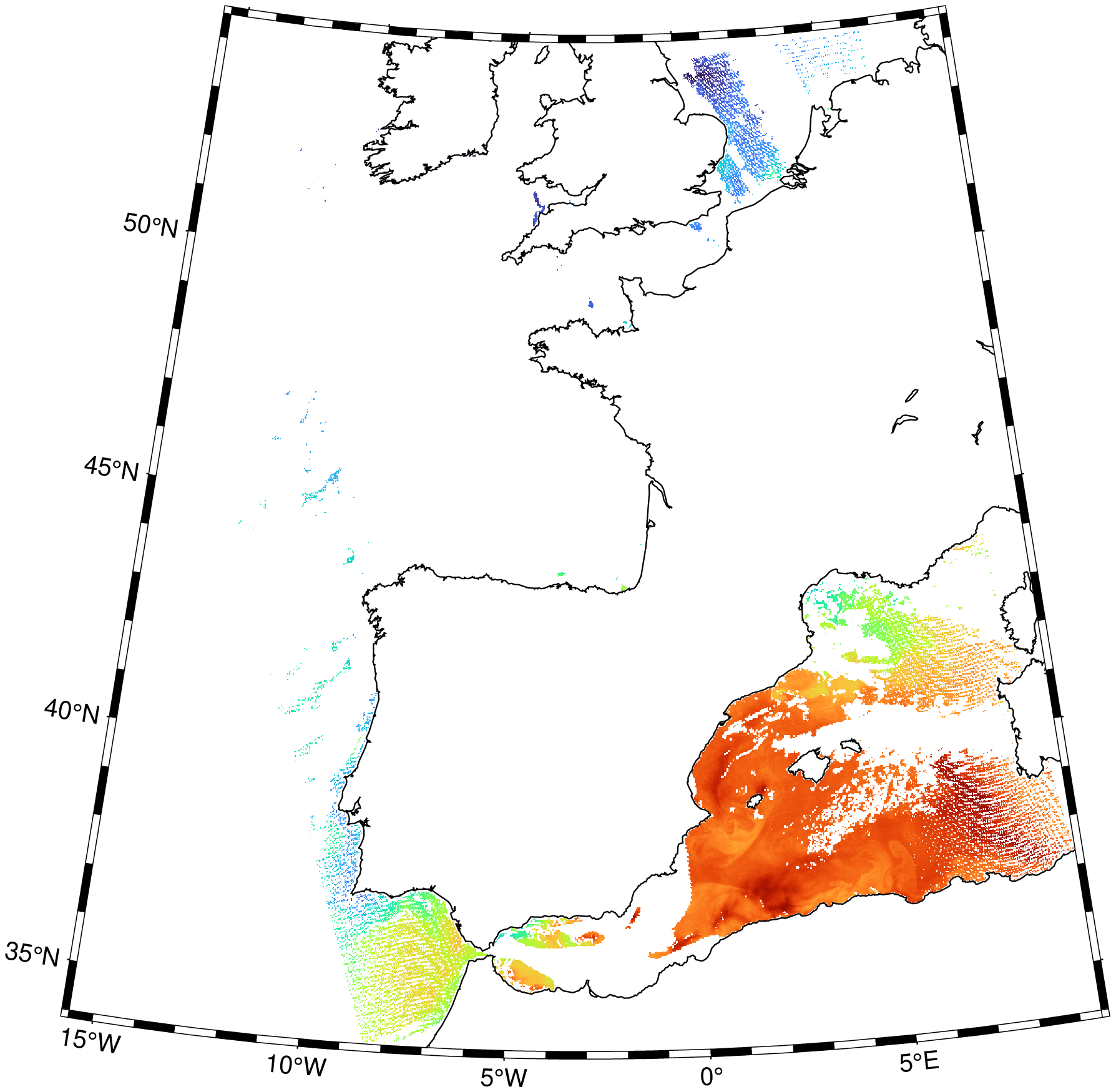
Note that since we used a grid step 0f 0.01 for the interpolation and this value is very close to the MODIS maximum spatial resolution, the left and right regions have beam spacings 2 to 5 times this and show many little holes. Do not confuse these little holes with the larger ones that are caused by cloud coverage. So we will recalculate the grid at increments of ~2 km and over the region that has the higher data density.
# Recompue at a inc=0.02 and over a sub-region
G = grid_at_sensor("C:/v/AQUA_MODIS.20210805T131001.L2.SST.NRT.nc", "sst", region=(-13,10,33.8,44.5), inc=0.02);
# Make a nicer image with illumination.
imshow(G, proj=:guess, coast=true, shade=true, title="Sea Surace Temperature", colorbar=true)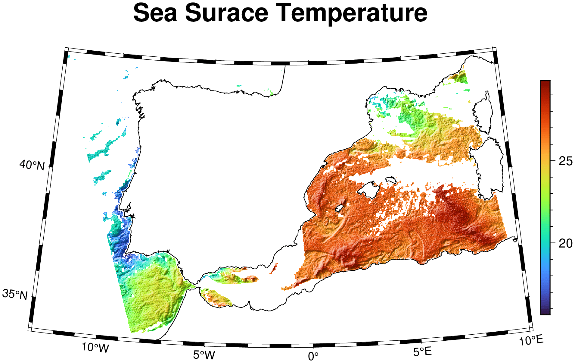
Download a Neptune Notebook here