Exploring a cube of Landsat 8 data
Here we will show examples of the type of things we can do with Landsat 8 data stored in a cube for better organisation and easyness of access.
The data was downloaded from EarthExplorer and comprises the scene with Product ID LC08_L1TP_204033_20210525_20210529_02_T1.
The cube was made with this instructions. Note that the LC08_L1TP_204033_20210525_20210529_02_T1_B is the part of the file names that is common to all band names.
using RemoteS, GMT
#cd(path-to-where-files-are-stored)
tplt = "LC08_L1TP_204033_20210525_20210529_02_T1_B";	# Template name
cube = cutcube(bands=[2,3,4,5,6,7,10], template=tplt, region=(485490,531060,4283280,4330290), save="LC08_L1TP_20210525_02_cube.tiff")```
This creates a 3D GeoTIFF file with the companion MTL file saved in it as Metadata. We can see the band info by running the reportbands function. That information is quite handy because we can, for example, just refer to the red band and it will figure out which layer of the cube contains the Red band.
using RemoteS, GMT
reportbands("LC08_L1TP_20210525_02_cube.tiff")
7-element Vector{String}:
 "Band 2 - Blue [0.45-0.51]"
 "Band 3 - Green [0.53-0.59]"
 "Band 4 - Red [0.64-0.67]"
 "Band 5 - NIR [0.85-0.88]"
 "Band 6 - SWIR 1 [1.57-1.65]"
 "Band 7 - SWIR 2 [2.11-2.29]"
 "Band 10 - Thermal IR 1 [10.6-11.19]"
So to start our exploration the best is to generate a true color image. The truecolor function knows how to do that automatically including the histogram contrast stretch.
Irgb = truecolor("LC08_L1TP_20210525_02_cube.tiff");
imshow(Irgb)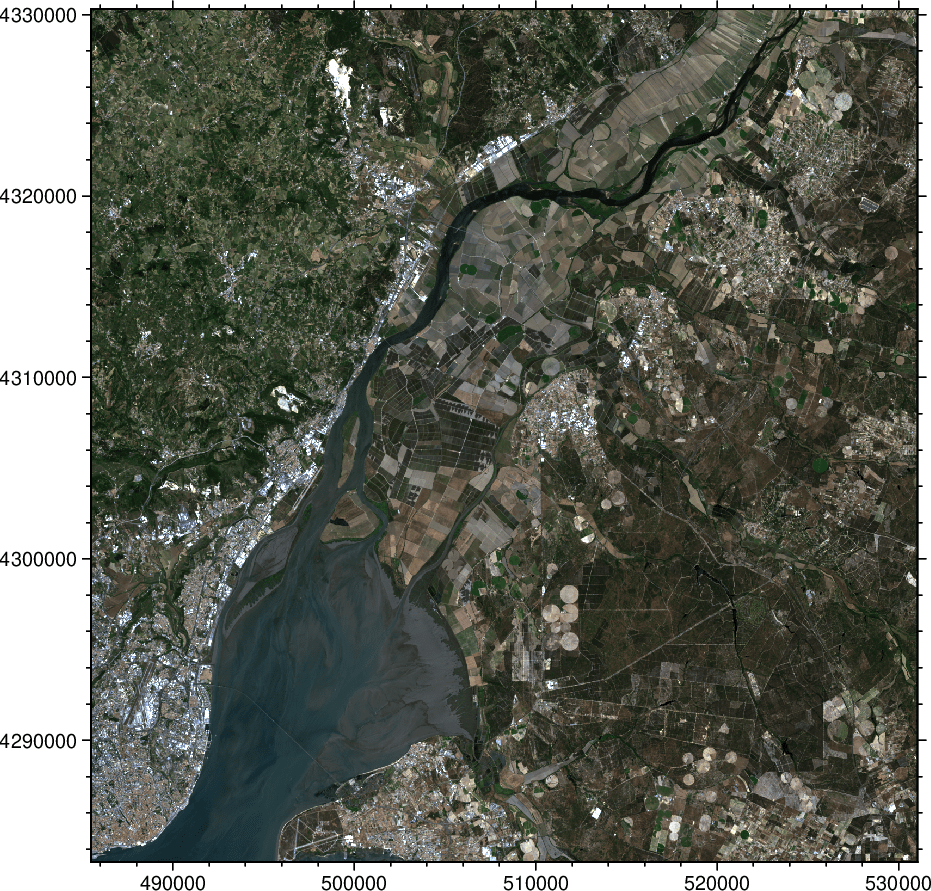
And we can compute the brightness temperature in Celsius at the Top of Atmosphere (TOA) from Band 10.
T = dn2temperature("LC08_L1TP_20210525_02_cube.tiff", band=10);
imshow(T, dpi=150, colorbar=true)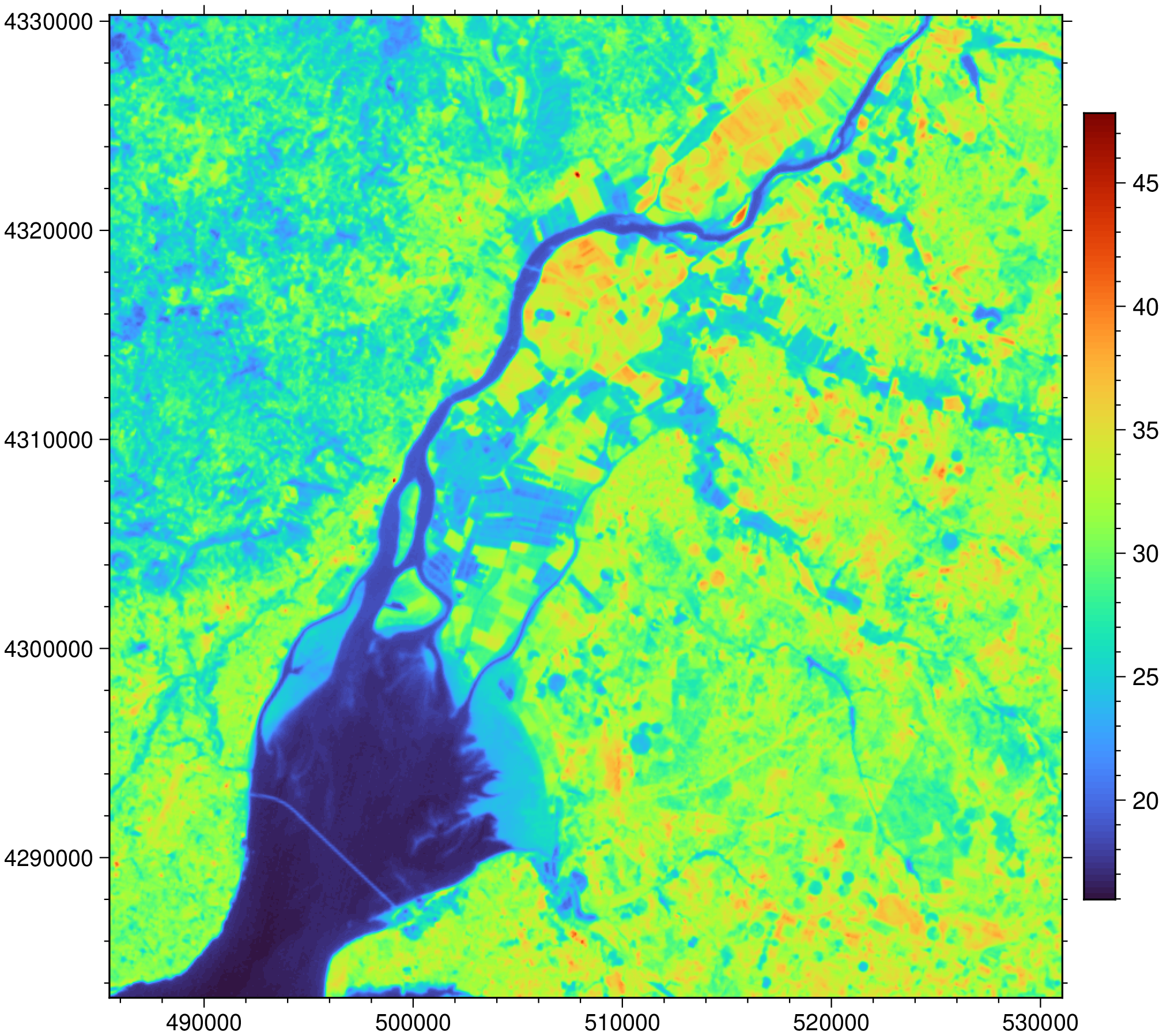
Or the Radiance TOA for the Blue band.
Btoa = dn2radiance("LC08_L1TP_20210525_02_cube.tiff", bandname="blue");
imshow(Btoa, dpi=150, color=:gray)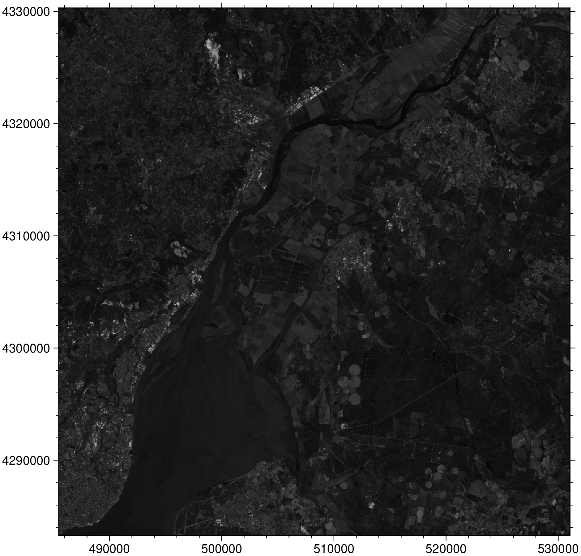
Hmmm, very dark. Let's look at its histogram.
histogram(Btoa, auto=true, show=true)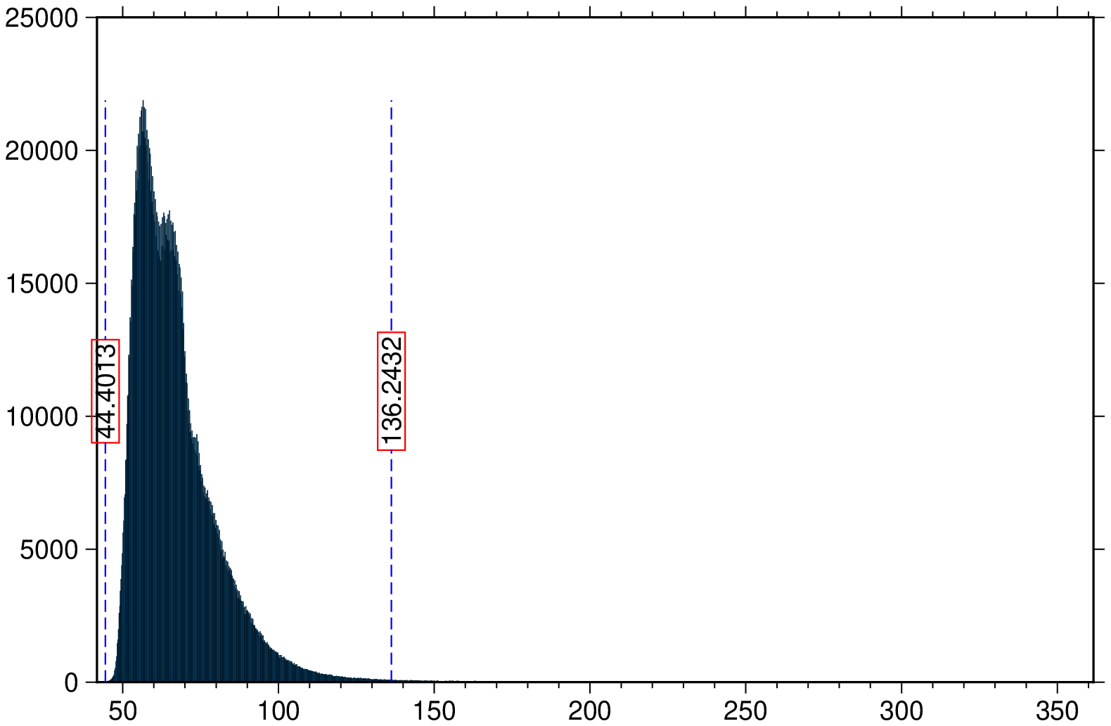
Yes, the data is very concentraded in the low numbers. We will need to apply a contrast stretch. To do that operation we will use the rescale function with the $stretch=true$ option that uses the limits displayed in the histogram figure above ans stretches the inner interval into [0 255] (by effect of the $type=UInt8$ option).
Btoa_img = rescale(Btoa, stretch=true, type=UInt8);
imshow(Btoa_img)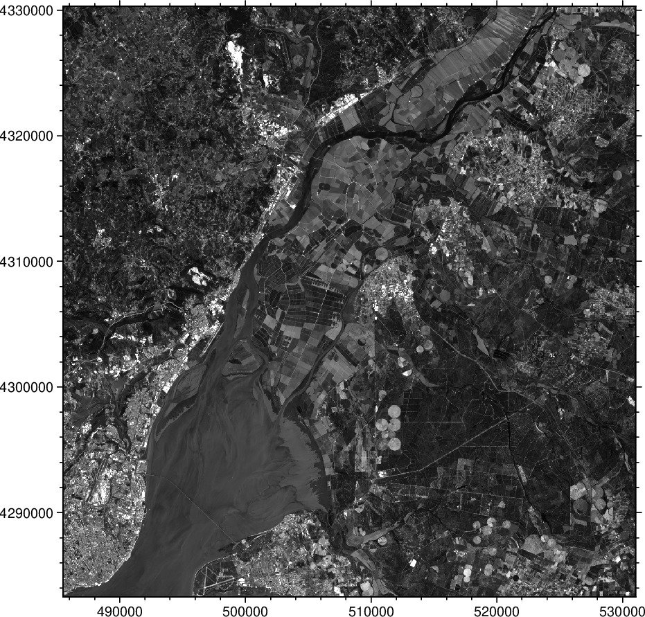
Now we are going to do the same for all Red, Green and Blue bands and compose the in a truecolor image. Repeating, we are going to compute the radiance at the top of atmosphere, retain only the data inside the parts of the histogram where it is more concentrated and create a true color image. To compute the radiance TOA we can do it all at once with the dn2radiance applied to the cube and, like before, create the RGB image with truecolor
cube_toa_rad = dn2radiance("LC08_L1TP_20210525_02_cube.tiff");
Irgb_toa = truecolor(cube_toa_rad);
imshow(Irgb_toa)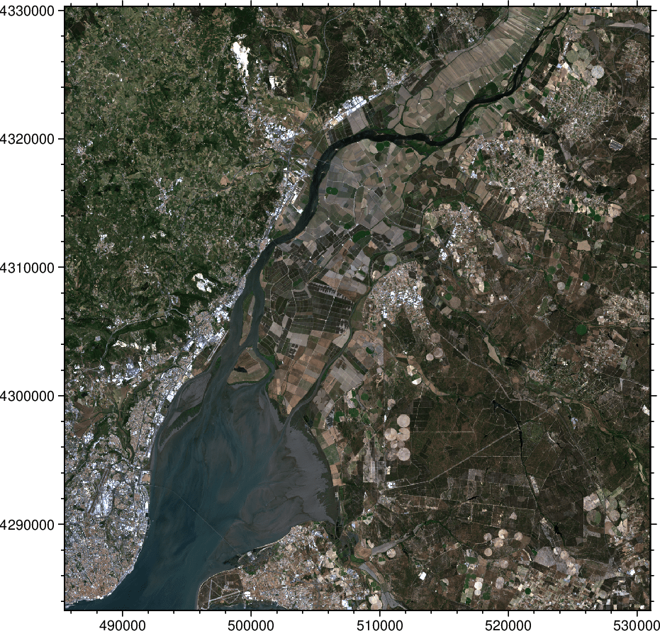
Hm, yes, very nice but it looks very much like the one obtained directly with the digital numbers. Indeed, it does but let us zoom in.
grdimage(Irgb, region=(502380,514200,4311630,4321420), figsize=8, frame=:bare)
grdimage!(Irgb_toa, figsize=8, projection=:linear, xshift=8, frame=:bare, show=true)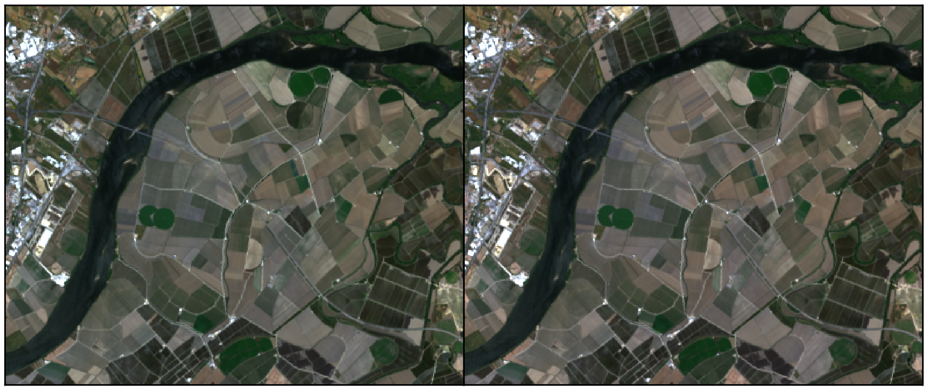
We can now clearly see that the image on the right, the one made the radiance TOA, has an higher contrast than the one made with data without any corrections.