Plot AQUA satellite tracks

Compute 1 day of AQUA satellite orbits starting at current local time. Note, this will be accurate for the month of September 2021. For other dates it needs an updated TLE. Note also that repeating the commands below will produce different results since the current local time is used as the starting point.

Orbits calculation rely on the SatelliteToolbox package(s). Orbits are calculated with the help of the so called Two Line Element files that unfortunatelly have accuracy validity quite short (around one month). They can be obtainded from the Space Track site.

using RemoteS, GMT, SatelliteToolboxTle, SatelliteToolboxPropagators, SatelliteToolboxTransformations

# The AQUA orbits TLE contents for the month of September 2021 
tle1 = "1 27424U 02022A   21245.83760660  .00000135  00000-0  39999-4 0  9997";
tle2 = "2 27424  98.2123 186.0654 0002229  67.6025 313.3829 14.57107527 28342";
orb = sat_tracks(tle=[tle1; tle2], duration="1D");

# The orbit track can be visualized with
imshow(orb,  proj=:Robinson, region=:global, coast=true)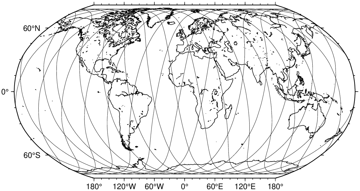

There is no point in plotting orbits for a lengthier duration because they would clutter the figure but we can compute them and display over a specific region on Earth.

# Compute orbits during 2 days at 15 seconds intervals
orb = sat_tracks(tle=[tle1; tle2], duration="2D", step=15);

# and plot them on my "vicinity"
D = clip_orbits(orb, [-20, 10, 30, 50]);

imshow(D, proj=:guess, coast=true, dpi=200)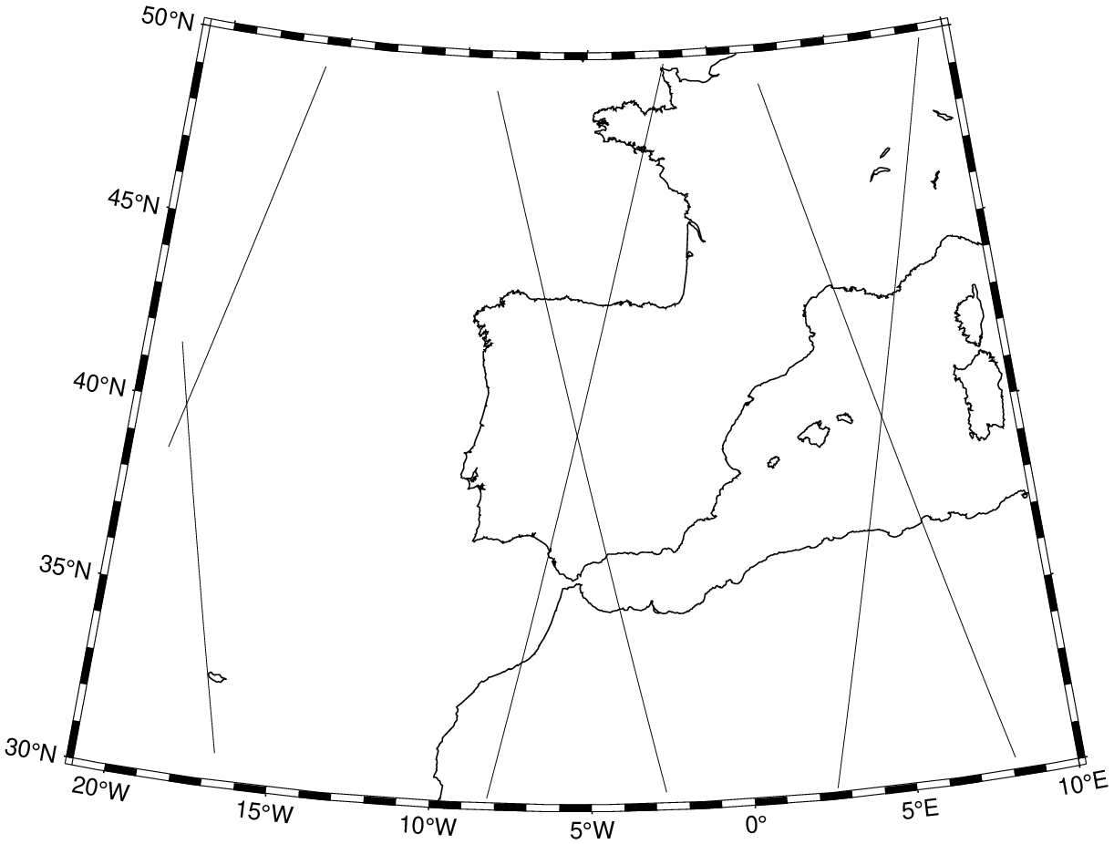

And imagine we would like to know the names of the AQUA scene files that cover a certain location? We can do it with the $findscenes$ function to which we must provide the location of interest, the satellite (currently only AQUA or TERRA), the duration of the search and if we want Chlorophyl-a concentration or Sea Surface Temperature (see function help for details).

# Get the scene names of data with Chlorophyl-a concentration covering
# the point (-8,36) and for two days before "2021-09-07T17:00:00"
tle1 = "1 27424U 02022A   21245.83760660  .00000135  00000-0  39999-4 0  9997";
tle2 = "2 27424  98.2123 186.0654 0002229  67.6025 313.3829 14.57107527 28342";
findscenes(-8,36, start="2021-09-07T17:00:00", sat=:aqua, day=true, duration=-2, oc=1, tle=[tle1, tle2])

	2-element Vector{String}:
	A2021251125500.L2_LAC_OC.nc
	A2021252134000.L2_LAC_OC.nc

Now you can download them from https://oceandata.sci.gsfc.nasa.gov/ob/getfile/A2021251125500.L2_LAC_OC.nc (but you will need to register first) and play with the grid_at_sensor function for interpolation and visualization.

Another cool thing we can do is to plot the area extent of the AQUA or TERRA scenes. We do it by first computing and orbit with a start and stop times and with increments of 1 minute (attention, this is an important factor). With that orbit we use the sat_tracks function to compute the polygons delimiting those areas.

using Dates

orb = sat_tracks(tle=[tle1; tle2], start=DateTime("2021-09-02T13:30:00"),
	stop=DateTime("2021-09-02T13:40:00"), step="1m");

Dsc = sat_scenes(orb, "AQUA");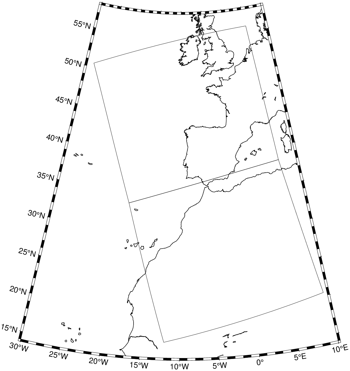

The scene names are stored in the header field of the Dsc GMTdatset

julia> Dsc[1].header

`AQUA_MODIS.20210902T133001.L2.SST.NRT.nc`

julia> Dsc[2].header

`AQUA_MODIS.20210902T133501.L2.SST.NRT.nc`

Download a Neptune Notebook here