(18) Volumes and Spatial Selections
To demonstrate potential usage of the programs gmtspatial, grdvolume and gmtselect we extract a subset of the Sandwell & Smith altimetric gravity field [1] for the northern Pacific and decide to isolate all seamounts that (1) exceed 50 mGal in amplitude and (2) are within 200 km of the Pratt seamount. We do this by dumping the 50 mGal contours to disk, then use gmtspatial that returns the mean location of the points making up each closed polygon, and then pass these locations to gmtselect, which retains only the points within 200 km of Pratt. We then mask out all the data outside this radius and use grdvolume to determine the combined area and (gravimetric) volumes of the chosen seamounts. Our illustration is presented in Figure 18 which also shows the automatic labeling offered by subplot.
#!/usr/bin/env bash
#		GMT EXAMPLE 18
#
# Purpose:	Illustrates volumes of grids inside contours and spatial
#		selection of data
# GMT modules:	gmtset, gmtselect, gmtspatial, grdclip, grdcontour, grdimage
# GMT modules:	grdmath, grdvolume, makecpt, coast, colorbar, text, plot
# Unix progs:	rm
#
gmt begin ex18
	# Use spherical gmt projection since SS data define on sphere
	gmt set PROJ_ELLIPSOID Sphere FORMAT_FLOAT_OUT %g
	# Define location of Pratt seamount and the 400 km diameter
	echo "-142.65 56.25 400" > pratt.txt
	gmt subplot begin 2x1 -A+JTL+o0.5c -Fs15c/9c -M0.5c/1c -R@AK_gulf_grav.nc -JM14c -B -BWSne
		gmt subplot set 0,0
		gmt makecpt -Crainbow -T-60/60
		gmt grdimage @AK_gulf_grav.nc -I+d
		gmt coast -Di -Ggray -Wthinnest
		gmt colorbar -DJCB+o0/1c -Bxaf -By+l"mGal"
		gmt text pratt.txt -D8p -F+f12p,Helvetica-Bold+jLB+tPratt
		gmt plot pratt.txt -SE- -Wthinnest
		# Then draw 10 mGal contours and overlay 50 mGal contour in green
		gmt subplot set 1,0
		gmt grdcontour @AK_gulf_grav.nc -C20
		# Save 50 mGal contours to individual files, then plot them
		gmt grdcontour @AK_gulf_grav.nc -C10 -L49/51 -Dsm_%d_%c.txt
		gmt plot -Wthin,green sm_*.txt
		gmt coast -Di -Ggray -Wthinnest
		gmt plot pratt.txt -SE- -Wthinnest
		rm -f sm_*_O.txt	# Only consider the closed contours
		# Now determine centers of each enclosed seamount > 50 mGal but only plot
		# the ones within 200 km of Pratt seamount.
		# First determine mean location of each closed contour and
		# add it to the file centers.txt
		gmt spatial -Q -fg sm_*_C.txt > centers.txt
		# Only plot the ones within 200 km
		gmt select -Cpratt.txt+d200k centers.txt -fg | gmt plot -SC0.1c -Gred -Wthinnest
		gmt plot -ST0.25c -Gyellow -Wthinnest pratt.txt
		# Then report the volume and area of these seamounts only
		# by masking out data outside the 200 km-radius circle
		# and then evaluate area/volume for the 50 mGal contour
		gmt grdmath pratt.txt POINT SDIST = mask.nc -fg
		gmt grdclip mask.nc -Sa200/NaN -Sb200/1 -Gmask.nc
		gmt grdmath @AK_gulf_grav.nc mask.nc MUL = tmp.nc
		area=$(gmt grdvolume tmp.nc -C50 -Sk -o1)
		volume=$(gmt grdvolume tmp.nc -C50 -Sk -o2)
		gmt text -M -Gwhite -Wthin -Dj0.7c -F+f14p,Helvetica-Bold+jLB -C8p <<- END
		> -149 52.5 14p 6.6c j
		Volumes: $volume mGal\267km@+2@+

		Areas: $area km@+2@+
		END
	gmt subplot end
gmt end show
rm -f sm_*.txt tmp.nc mask.nc pratt.txt center*
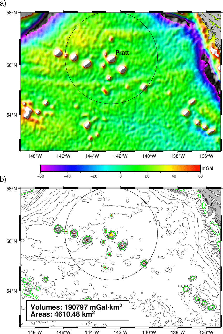
Volumes and geo-spatial selections.