Anatomy of a GMT figure¶

This tutorial will cover the fundamental concepts behind making figures with GMT, including starting a modern mode session, setting a region, drawing a map frame, choosing a projection, and adding simple elements (e.g., coastlines) to a map.

Let’s get started!

Creating a GMT session¶

In GMT modern mode, all processing and plotting commands are contained within a code block starting with gmt begin and ending with gmt end.

In the Jupyter Notebook, we use cell magic (%%bash) to show that the cell should be executed as a bash script. In a regular bash script, you would instead put #!/usr/bin/env bash at the top of your script. We also use the IPython.display.Image class to show the figures created by the GMT sessions in the Jupyter notebook.

# Load the class first. This only needs to be run once
from IPython.display import Image

%%bash

# Start a modern mode session
gmt begin # optionally append a session name (e.g., 'gmtsession') and one or more comman-separated figure formats (e.g., 'png,pdf')
    # Any number of gmt and UNIX commands can go between 'gmt begin' and 'gmt end'
# End a modern mode session
gmt end # optionally append 'show' to display the outputs

Drawing coastlines¶

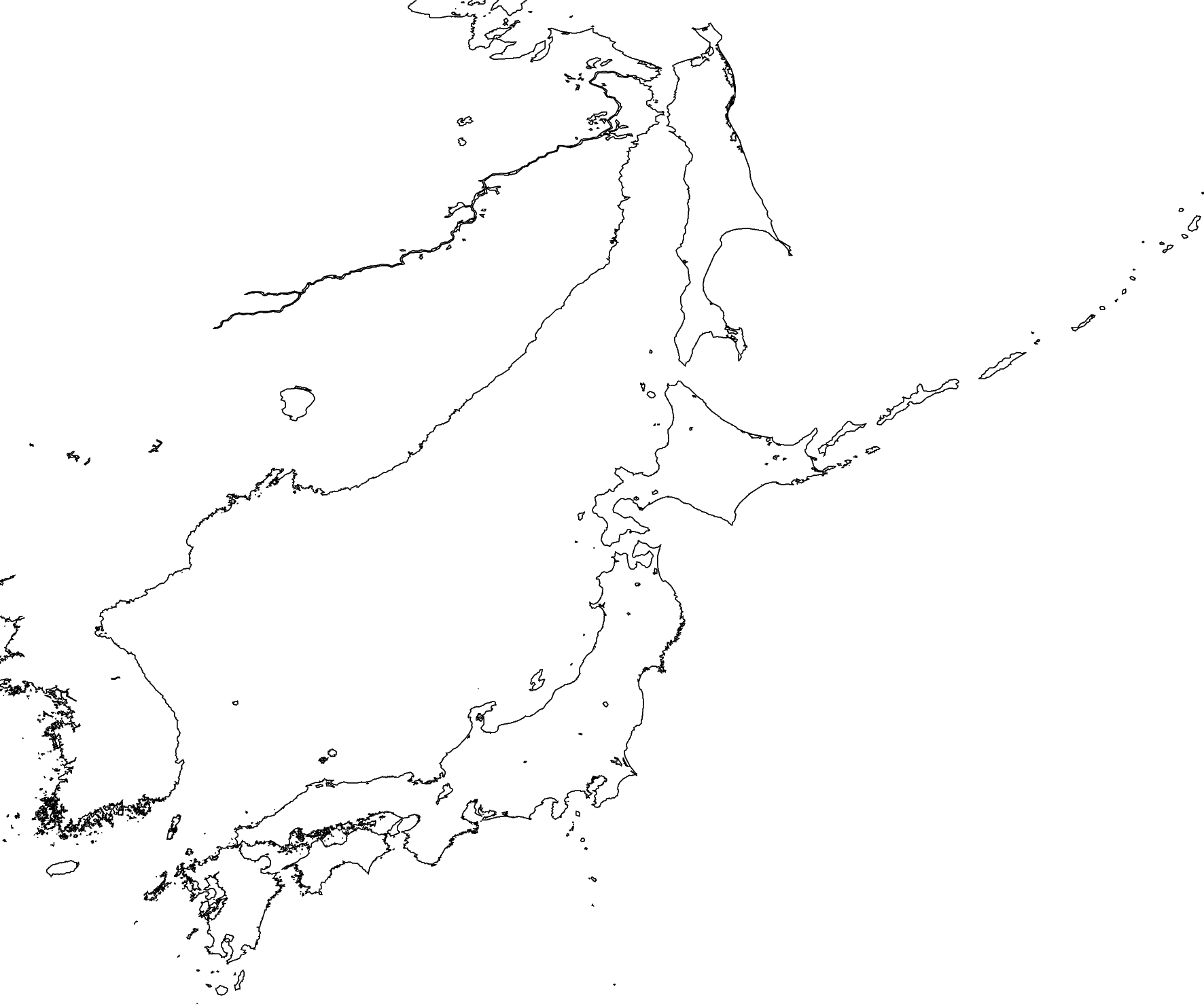
We need to specify the geographic bounding box that contains the data/features we want to plot. This bounding box is set using the -R common option and it has the format of a string containing the West/East/South/North (WESN) coordinates of the bounding box. We can lay down the coastlines for this region using -W option of the coast module.

%%bash

gmt begin coastlines png
    gmt coast -R125/155/30/55 -W
gmt end

Image('coastlines.png', width=300)

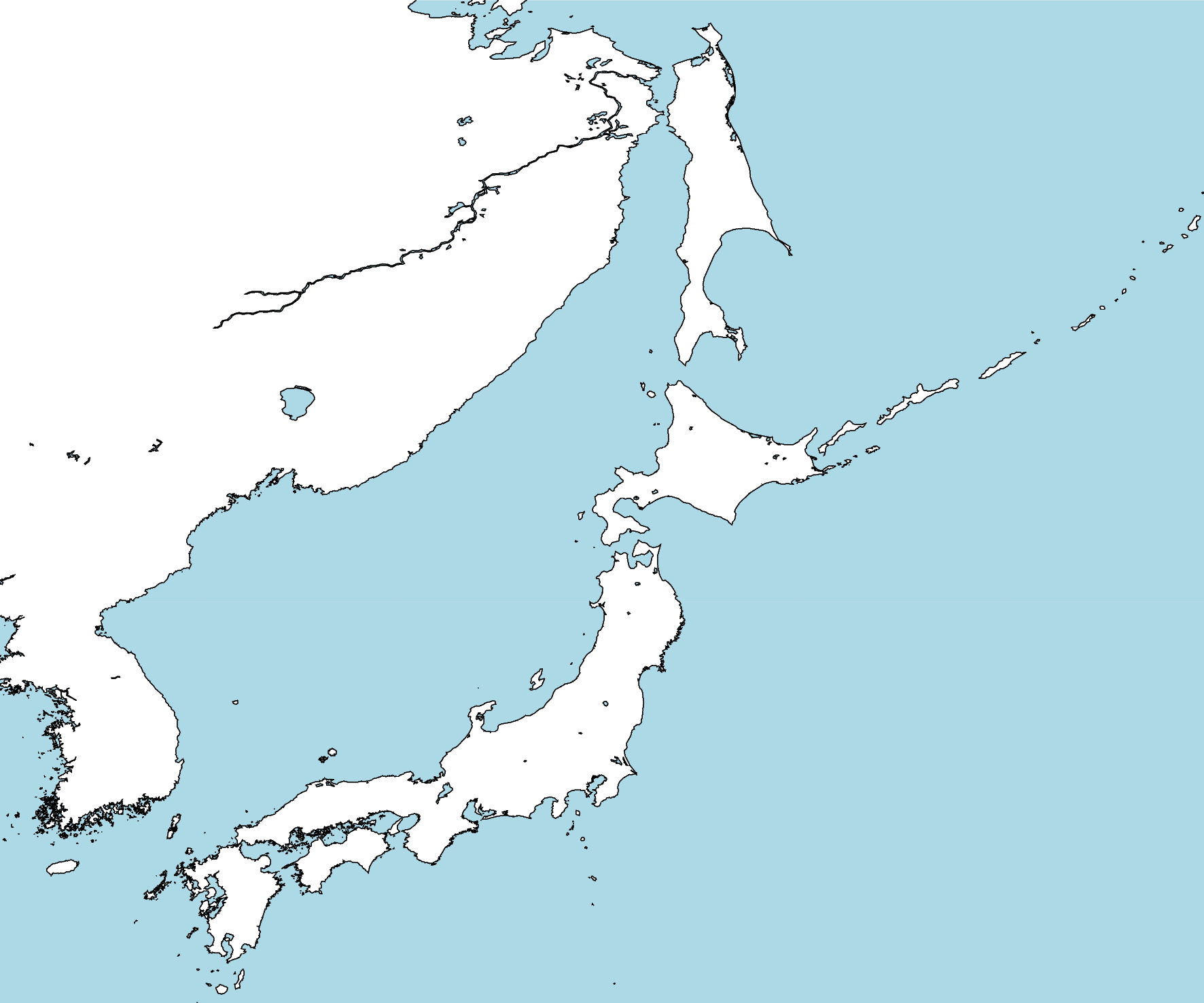
Beyond the outlines, we can also color the land and water regions to make them stand out. Lets start with the water using the -S option of the coast module.

%%bash

gmt begin coastlines png
    gmt coast -R125/155/30/55 -W -Slightblue
gmt end

Image('coastlines.png', width=300)

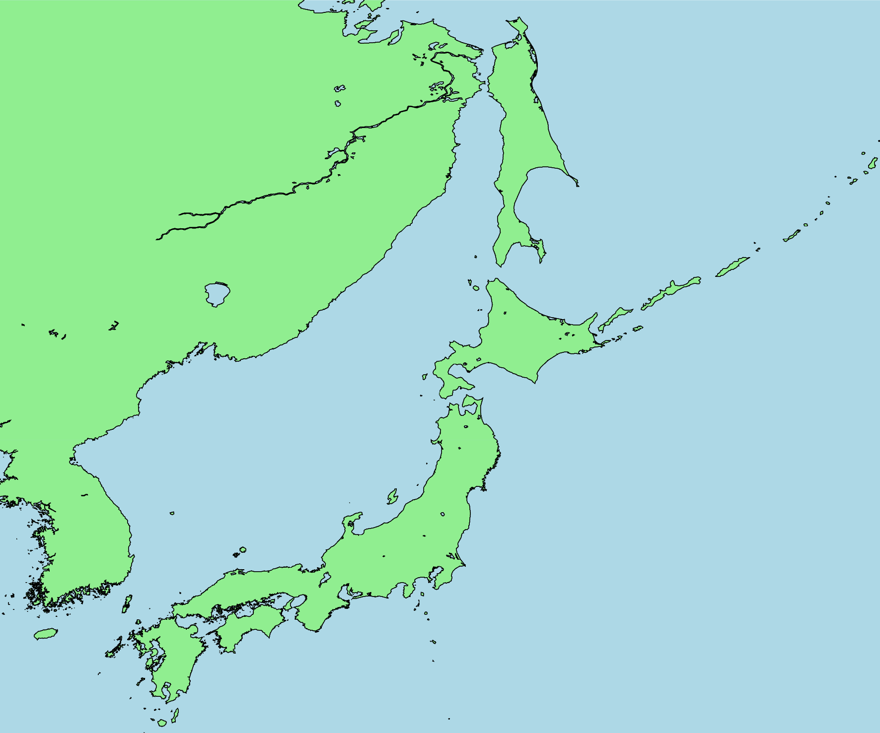
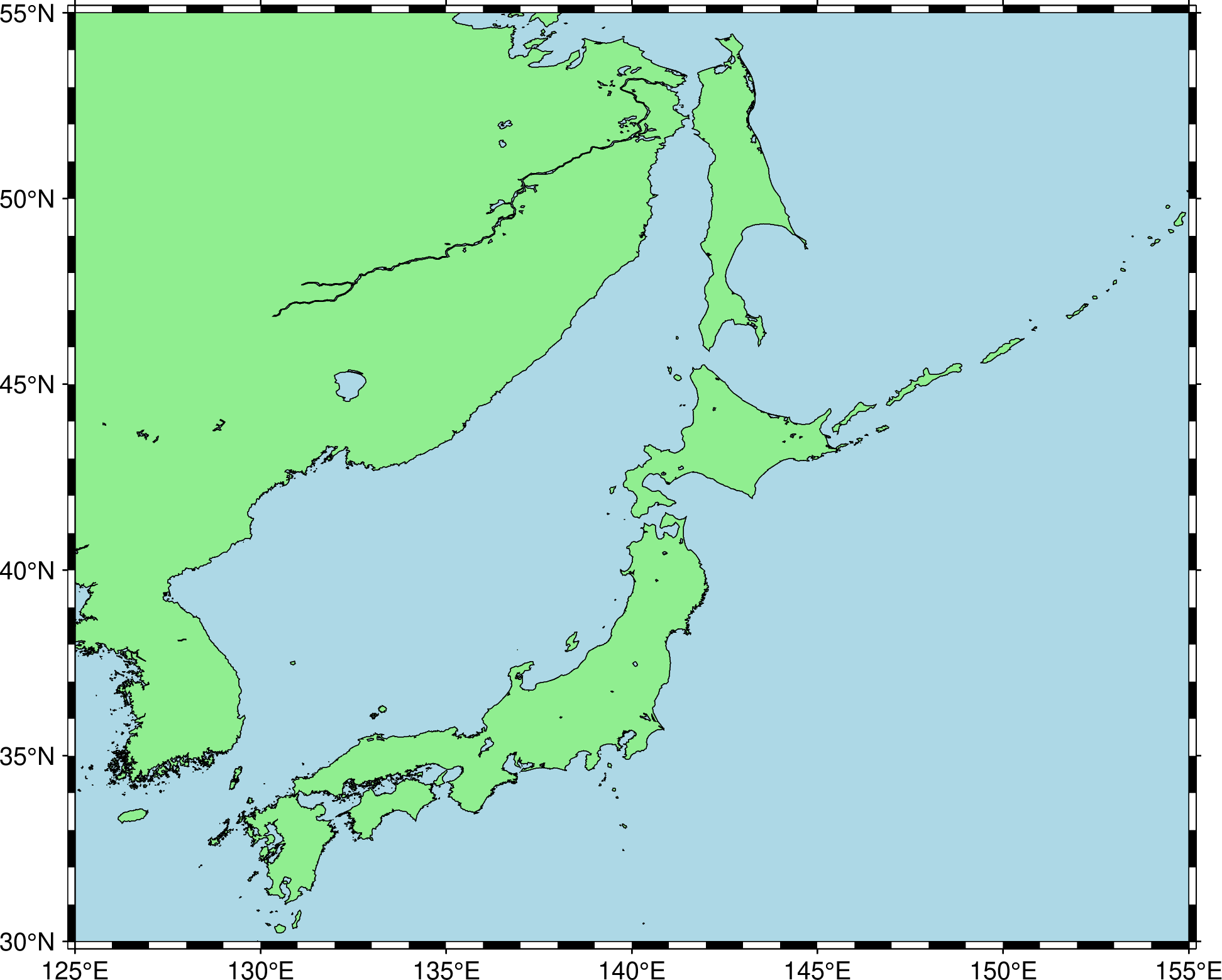
And now add the land in a light green color using the -G option.

%%bash

gmt begin coastlines png
    gmt coast -R125/155/30/55 -W -Slightblue -Glightgreen
gmt end

Image('coastlines.png', width=300)

Alright, now we have a lovely figure with colored land and water plus some shorelines. But what are the coordinates associated with this map? Lets add a map frame to find out.

Drawing a map frame¶

Adding a nice frame with coordinates, ticks, and labels is one of the jobs of the basemap module. Here, we’ll use it to add automatic annotations ("a") around the figure we just made above. It will be the last item we lay on our figure canvas to guarantee that it sits above any other plot elements.

%%bash

gmt begin coastlines png
    gmt coast -R125/155/30/55 -W -Slightblue -Glightgreen
    gmt basemap -Ba
gmt end

Image('coastlines.png', width=300)

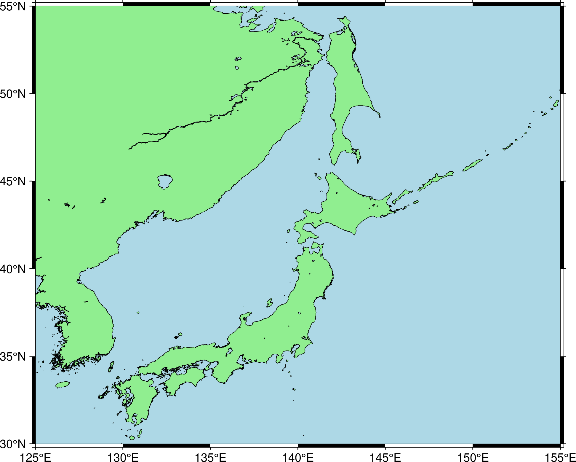
Notice that the coordinates are automatically recognized as longitude and latitude and the tick spacing is chosen sensibly as well.

There are many different ways in which we can customize the frame, from the ticks to the interval to the labels. Here we’ll only cover a few of the most common things you’d want to do. Starting with…

Adding minor ticks¶

The ticks with annotations are known as “major ticks” (controlled by the "a") value. You can also add automatic “minor ticks” which have a smaller interval and won’t have annotations by adding "f" to the frame argument.

%%bash

gmt begin coastlines png
    gmt coast -R125/155/30/55 -W -Slightblue -Glightgreen
    gmt basemap -Baf
gmt end

Image('coastlines.png', width=300)

The frame is now set to have both annotations and minor ticks, both of which are optional (so frame="f" would mean only having minor un-annotated ticks). Try it out!

Adding grid lines¶

Grid lines are enabled by adding "g" to frame, just like we did for minor ticks. Again you can mix and match the three arguments "a", "f", and "g".

%%bash

gmt begin coastlines png
    gmt coast -R125/155/30/55 -W -Slightblue -Glightgreen
    gmt basemap -Bafg
gmt end

Image('coastlines.png', width=300)

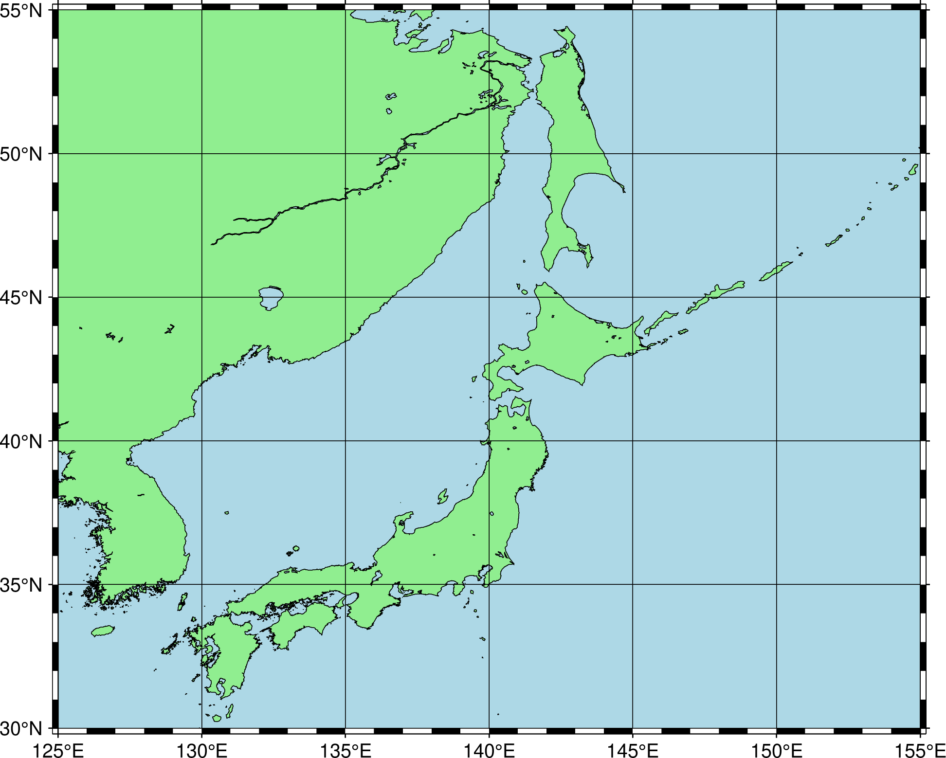
By default the spacing of the grid lines is the same as the annotated major ticks.

Note

Adding a frame with grid lines before you plot the colored land and water or an image will hide the grid lines beneath the subsequent plot. Make sure you put the call to basemap last to avoid this.

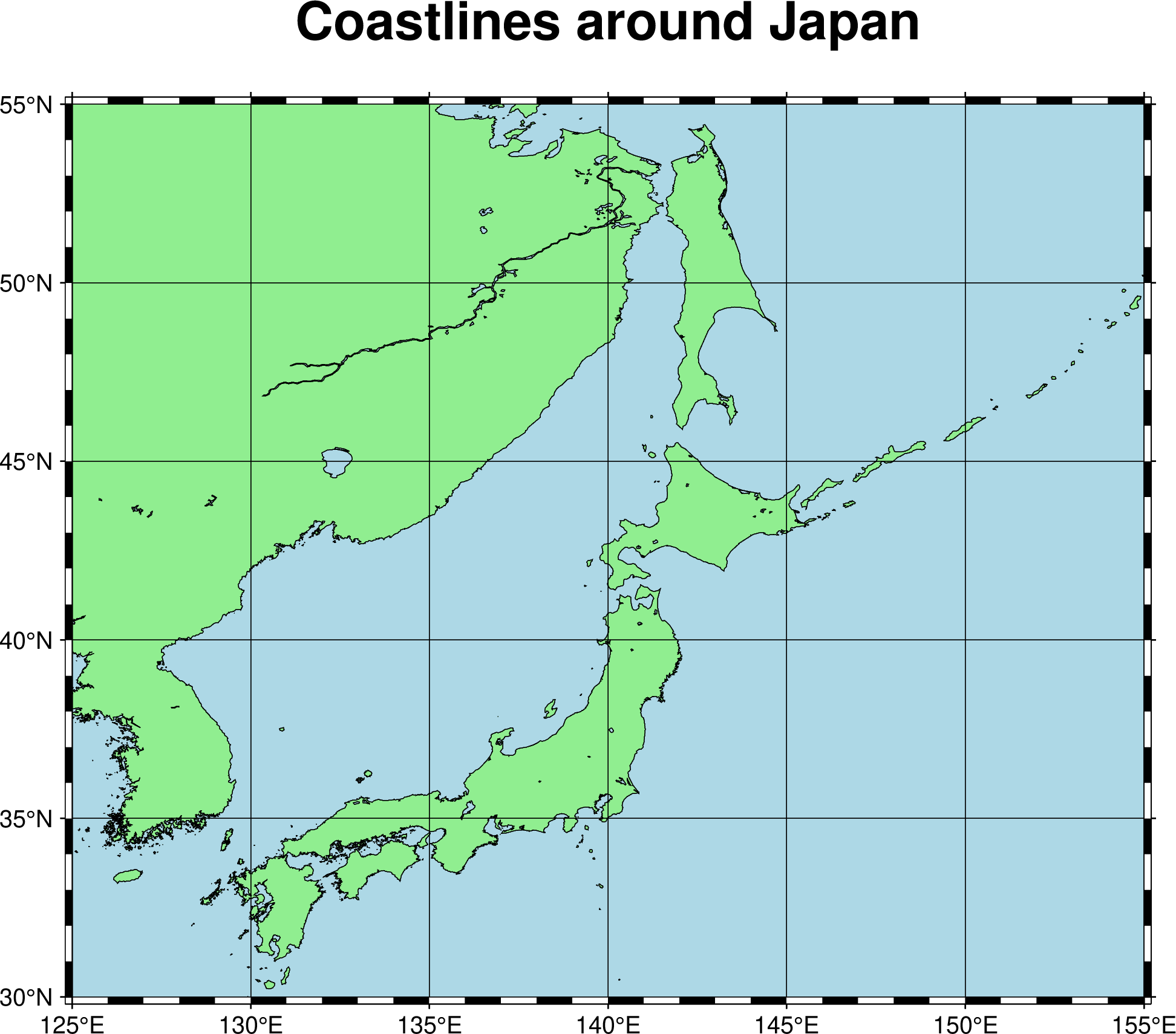
Adding a title¶

To add a title to the figure, we need to pass in more than one -B arguments to basemap. The extra argument for adding a title is a string with the format "+tMy title goes here".

%%bash

gmt begin coastlines png
    gmt coast -R125/155/30/55 -W -Slightblue -Glightgreen
    gmt basemap -Bafg -B+t'Coastlines around Japan'
gmt end

Image('coastlines.png', width=300)

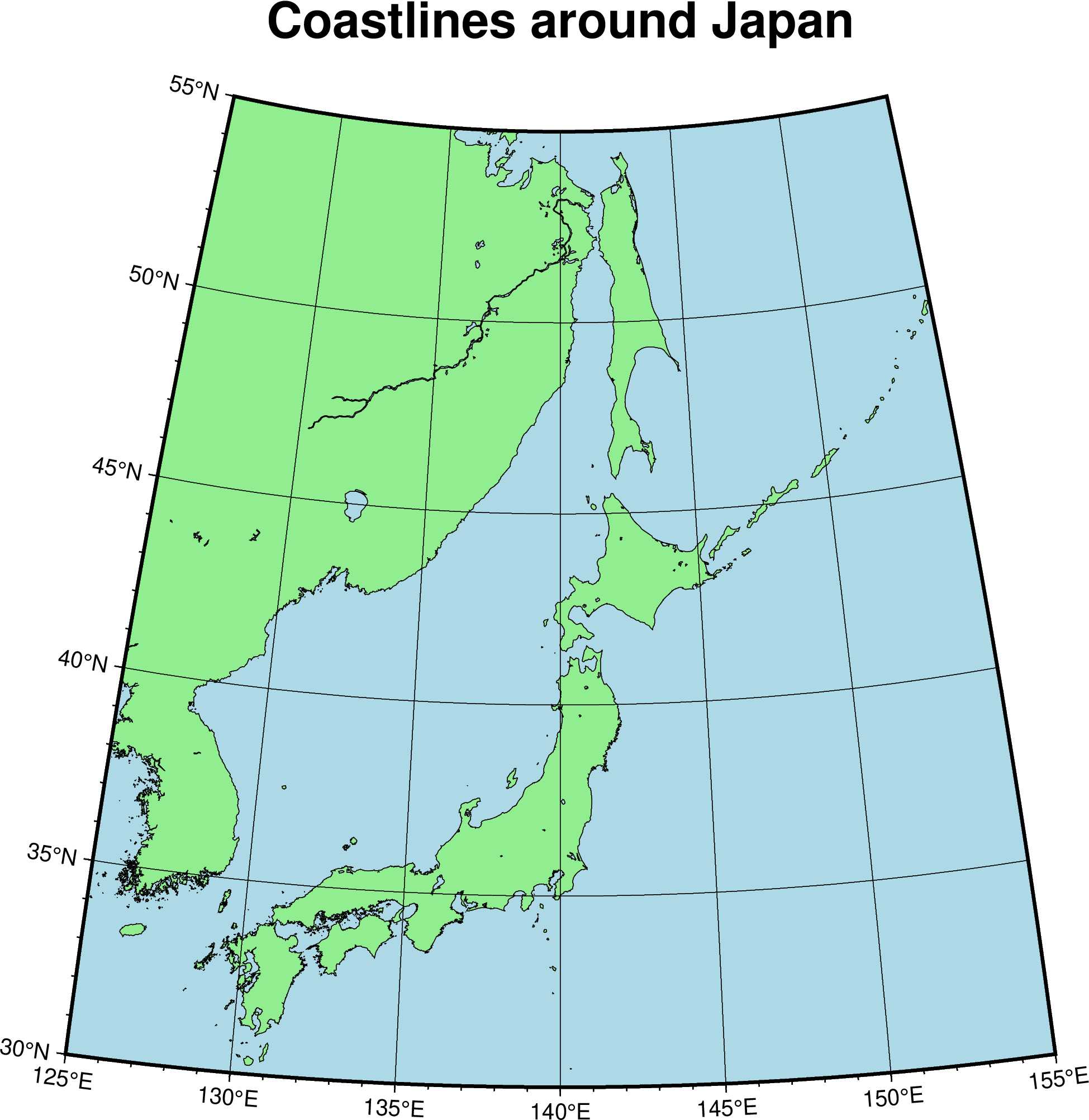
Choosing a projection¶

In modern mode, GMT will chose a default projection based on the input data. Many projections are supported, which may often be better suited for your plots that the default selection (particularly around the polar regions or for larger global maps).

For our case, let’s go with a Cassini projection. To specify this, we need to pass an argument for the -J option to the first plot method we call. The projection specification is a string starting with a 1-letter code for the projection followed by the projection arguments (particular to each projection) and finishing off with the physical width of the figure (in centimeters or inches, usually). For the Cassini projection, this is what it would look like: -JC142.5/40/15c in which C is for Cassini projection, 142.5 is the central longitude of the projection set to the center of our region, 40 is the same for the central latitude, and 15c means the plot will be 15 centimeters wide on the page (this influences the relative size of fonts and tick labels).

%%bash

gmt begin coastlines png
    gmt coast -R125/155/30/55 -W -Slightblue -Glightgreen -JC140/40/15c
    gmt basemap -Bafg -B+t'Coastlines around Japan'
gmt end

Image('coastlines.png', width=300)

GMT for Geodesy

Anatomy of a GMT figure

Contents